Natural Gas
Abstract
Natural Gas is a form of hydrocarbon that is strongly related to oil. In the United States it is widely used for space-heating and to generate electricity. However, even though gas production peaked in the US in 1971, it has been resurrected through the shale gas boom. Moreover, natural gas remains the third most widely used energy source in the world, ranking just below coal.
Natural gas is another form of hydrocarbon that is strongly related to oil. Normally, natural gas is produced from reservoirs that are separate and distinct from oil reservoirs, although there is always some gas produced form oil reservoirs as well. In the United States, as well as the rest of the world, natural gas is widely used for: space heating; to generate electricity; as an industrial fuel source; as a feedstock for petrochemicals; and, as a feedstock to make gasoline and other transportation fuels. In Chapter 5, gas production in the United States was briefly discussed as an analogy for world oil production. Even though gas production had already peaked in the United States in early 1973, it has reversed this decline and has now reached a new production peak and is still increasing. Natural gas is the third most widely used energy source in the world, just below coal. It has a very bright future with increasing importance, both in the world and in the United States.
Natural gas consists primarily of methane but can have other components. Some of these components are beneficial to its heat content such as ethane, propane, butane, and other longer chain hydrocarbons. Other components are considered impurities because they are undesirable components such as nitrogen, carbon dioxide, and hydrogen sulfide. They must be removed before the gas can be sold. Due to the fact that all oil and gas reservoirs contain residual water saturation, gas must also be dried before it can be put in a pipeline to be transported to market. Depending on the reservoir and production conditions, the produced gas can contain up to 150 pounds of water per million cubic feet of gas. The usual pipeline specifications are that gas must contain no more than 7 pounds of water per million cubic feet before it can be transported by pipeline. If this specification is not met, it leads to corrosion in the pipeline as well as water pooling in low spots in the line. Impurities such as carbon dioxide and hydrogen sulfide are acidic gasses and, if they are not removed, they also lead to corroded lines as well as other dangerous conditions.
Natural gas also tends to contain small amounts of ethane, propane, butane, and other longer chain hydrocarbons. These molecules have higher heat content than methane, so there is some benefit in letting these components remain in the gas; however, this can lead to some disadvantages which necessitate their removal. First, under certain conditions, the heavier hydrocarbons can also drop out of the gas during transportation in the pipeline and then they pool in low spots impeding the flow of the gas. They can also cause the gas to burn hotter than methane which, for certain applications, is not desired because it can lead to degradation of the equipment. Consequently, the longer chain hydrocarbons are usually reduced to meet pipeline specifications for gas.
The World Picture
Worldwide natural gas production has increased from 97 billion cubic feet (BCF) per day in 1970 to 309 BCF per day in 2010, as shown in Figure 6.1. During that time, the annual growth rate has been a steady 2.75%. The only decrease in supply and demand occurred due to the world financial crisis in 2008. Natural gas meets 21.4% of the world energy supply, third only to oil and coal. In the United States, it is responsible for 24.3% of the energy supply, second only to oil. The largest gas-producing countries in the world, with their daily production rate, are shown in Table 6.1. Their reserves are shown in Table 6.2 and their reserve life is shown in Table 6.3. Remember, reserve life is calculated by dividing the reserves by the daily production rate and converting the answer (given in days) to years.
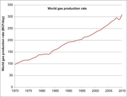
Table 6.1
Largest Gas Producers in the World (BCF per Day).
| 1 | USA | 59.12 |
| 2 | Russia | 56.98 |
| 3 | Canada | 15.46 |
| 4 | Iran | 13.40 |
| 5 | Qatar | 11.29 |
| 6 | Norway | 10.29 |
| 7 | China | 9.36 |
| 8 | Saudi Arabia | 8.12 |
| 9 | Indonesia | 7.93 |
| 10 | Algeria | 7.78 |
| 11 | Netherlands | 6.82 |
| 12 | Malaysia | 6.43 |
| 13 | Egypt | 5.93 |
| 14 | Uzbekistan | 5.72 |
| 15 | United Kingdom | 5.53 |
| 16 | Mexico | 5.35 |
| 17 | United Arab Emirates | 4.94 |
| 18 | India | 4.92 |
| 19 | Australia | 4.87 |
| 20 | Trinidad & Tobago | 4.10 |
| 21 | Turkmenistan | 4.10 |
| 22 | Argentina | 3.88 |
| 23 | Pakistan | 3.82 |
| 24 | Thailand | 3.51 |
| 25 | Nigeria | 3.25 |
| 26 | Kazakhstan | 3.25 |
| 27 | Venezuela | 2.76 |
| 28 | Oman | 2.62 |
| 29 | Bangladesh | 1.94 |
| 30 | Ukraine | 1.79 |
Table 6.2
Largest Gas Reserves in the World (TCF).
| 1 | Russia | 1580.77 |
| 2 | Iran | 1045.67 |
| 3 | Qatar | 894.22 |
| 4 | Turkmenistan | 283.58 |
| 5 | Saudi Arabia | 283.06 |
| 6 | USA | 272.51 |
| 7 | United Arab Emirates | 212.97 |
| 8 | Venezuela | 192.70 |
| 9 | Nigeria | 186.89 |
| 10 | Algeria | 159.06 |
| 11 | Iraq | 111.87 |
| 12 | Indonesia | 108.40 |
| 13 | Australia | 103.12 |
| 14 | China | 99.15 |
| 15 | Malaysia | 84.65 |
| 16 | Egypt | 78.05 |
| 17 | Norway | 72.11 |
| 18 | Kazakhstan | 65.18 |
| 19 | Kuwait | 63.00 |
| 20 | Canada | 61.00 |
| 21 | Uzbekistan | 55.08 |
| 22 | Libya | 54.70 |
| 23 | India | 51.22 |
| 24 | Azerbaijan | 44.86 |
| 25 | Netherlands | 41.45 |
| 26 | Ukraine | 33.02 |
| 27 | Pakistan | 29.09 |
| 28 | Oman | 24.37 |
| 29 | Vietnam | 21.79 |
| 30 | Romania | 21.02 |
Table 6.3
Gas Reserve Life (Years).
| 1 | Iraq | 2534 |
| 2 | Qatar | 217 |
| 3 | Iran | 214 |
| 4 | Venezuela | 191 |
| 5 | Turkmenistan | 190 |
| 6 | Nigeria | 157 |
| 7 | Kuwait | 154 |
| 8 | United Arab Emirates | 118 |
| 9 | Libya | 98 |
| 10 | Saudi Arabia | 95 |
| 11 | Azerbaijan | 84 |
| 12 | Yemen | 78 |
| 13 | Russia | 76 |
| 14 | Vietnam | 66 |
| 15 | Australia | 58 |
| 16 | Algeria | 56 |
| 17 | Kazakhstan | 55 |
| 18 | Romania | 54 |
| 19 | Ukraine | 50 |
| 20 | Peru | 49 |
| 21 | Indonesia | 37 |
| 22 | Malaysia | 36 |
| 23 | Egypt | 36 |
| 24 | Syria | 33 |
| 25 | Poland | 29 |
| 26 | China | 29 |
| 27 | Brazil | 29 |
| 28 | India | 29 |
| 29 | Myanmar | 28 |
| 30 | Uzbekistan | 26 |
From these figures, it can be seen that the United States is the largest gas producer in the world and the sixth largest in reserves. It does not appear on the list of top countries in terms of reserve life because its reserve life is less than 13 years, which puts it thirty-ninth on the world list. This list, however, is based on proved reserves and later you will see that the United States has a lot more gas that remains unproven because many more wells have to be drilled to prove these additional reserves.
As with oil reserves, all the countries on the reserve life list that have more than 25 years supply, have the capacity to increase their production if and when the world needs it. There are many more countries that have large spare gas production capacity than have spare oil production capacity. Natural gas remains an underutilized energy source. As in the United States, there is a lot of gas around the world that is still waiting to be discovered and produced.
The trade in natural gas is not as active as oil. This is because the most cost effective way to transport gas is by pipeline. This limits the gas import/export trade. There is a modest but growing liquefied natural gas (LNG) trade, but most of the international trade is still done by pipeline where possible. There are large pipelines supplying natural gas to Europe from Russia and smaller lines running from Algeria to Europe and from Canada to the United States and also between various South American countries. Most gas is produced and used locally.
Liquefied Natural Gas
The import/export trade in natural gas is not nearly as large as the oil trade because it is more difficult to export gas. If the importing country lies close to the exporting country and they are connected by land, the gas can be transported by pipeline. Large bore pipelines exist between Russia and Europe, Algeria and Europe, Canada and the United States and between some South American countries, particularly Bolivia, Brazil, Chile, and Argentina. While oil can be readily shipped over the ocean by tanker, natural gas must first be liquefied by refrigeration to be shipped the same way. This is expensive and adds to the cost of the gas. Nevertheless, there is a growing trade in LNG.
In order to be liquefied, natural gas must be cooled to about − 259 °F at atmospheric pressure. This results in the condensation of the gas into liquid form, which takes up about one six hundredth (0.167%) of the volume of natural gas vapor. Liquefaction also has the advantage of removing the heavier hydrocarbon molecules (particularly ethane, propane, and butane) and impurities such as nitrogen, carbon dioxide, sulfur, and water. This results in LNG that is almost pure methane.
LNG is typically transported by a specialized tanker with insulated walls. It is maintained in liquid form by auto-refrigeration, a process in which the LNG is kept at its boiling point so that any heat that is conducted through the tanker walls is countered by the latent heat of vaporization, energy that is lost from the LNG as it vaporizes. The vapor is vented out of storage and then burned to provide motive power for the tanker. Once it is delivered to a port, the LNG must be vaporized again before it can be transported and burned.
There is some misplaced public concern about the safety of LNG facilities, misplaced because they actually have a remarkably good safety record over a long period of usage. In its liquid state, LNG is not explosive and cannot burn. For LNG to burn, it must first vaporize, then mix with air in the right proportions—(5-15%) and then be ignited. In the case of a leak, LNG vaporizes rapidly, turning back into a gas (methane) and mixing with air. If this mixture is within the flammable range, there is risk of ignition which, if confined, could create an explosion. If the leaking gas is vented to an unconfined space, it can burn but not explode.
There have never been any explosions or significant accidents aboard LNG tankers which have sailed more than 100 million miles without incident. In the past 65 years, there has only been one significant accident at an LNG re-vaporization facility. On October 6, 1979, at the Cove Point LNG facility in Lusby, Maryland, a pump seal failed. This allowed gas vapors to enter an electrical conduit. The explosion that followed would have been prevented by the automatic activation of a circuit breaker, but a worker had switched off the circuit breaker and the gas vapors ignited. One worker was killed, another was severely injured, and there was major damage to the building. This accident led to tougher safety codes for the operation of LNG facilities in the United States.
A more serious accident occurred on January 19, 2004 at one of the natural gas liquefaction units in Skikda, Algeria. A leak occurred in the hydrocarbon refrigerant system, forming a flammable vapor that was sucked into the inlet of the combustion fan of a steam boiler. The hydrocarbon refrigerant acted as increased fuel to the boiler, causing increased pressure within the steam-generating equipment. The rapidly rising pressure quickly exceeded the capacity of the boiler’s safety valve and the steam drum ruptured, tearing apart the boiler. The flames from the ruptured boiler ignited the leaking refrigerant gas, which was confined by the equipment and structures in the area, producing an explosion and a fire. The explosion, along with the shrapnel from the ruptured steam drum, caused further damage to the piping and pressure vessels in the immediate area, leading to additional flammable fluid release. The fire took 8 h to extinguish. The explosions and fire destroyed a portion of the petrochemical complex and caused 27 deaths and injuries to 72 people. No one outside the plant was injured nor were the LNG storage tanks or the marine facilities damaged by the explosions. Even though the accident occurred in Algeria, the U.S. Federal Energy Regulatory Commission (FERC) and the U.S. Department of Energy (DOE) conducted their own investigation of the accident and a joint report was issued in April 2004. The findings of the report were that:
• There were ignition sources in the process area
• There was a lack of “typical” automatic equipment shutdown devices required by U.S. LNG design codes, and
• There was a lack of hazard detection devices.
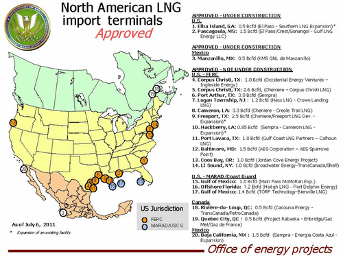
There are currently 10 LNG unloading and re-vaporization facilities in operation in the United States (see Figure 6.2). Sixteen more have been approved for construction and, of these, two are currently under construction. Many of these were approved prior to new supplies of natural gas becoming available in the United States, and it is unlikely that all of them will actually be built. Some of them might be converted into LNG export facilities. Figure 6.3 shows the location of these 16 facilities and 4 others located in Mexico and Canada. Due to the oversupply of the natural gas market in the United States, some LNG that is currently being delivered to the U.S. LNG terminals is now being re-exported. These re-exports occur when foreign LNG shipments are offloaded into above-ground U.S. storage tanks located on-site at the terminals. They are then subsequently reloaded onto tankers for delivery to other countries.

Due to the reduction of LNG imports into the United States, some of the import facilities are being used for temporary storage of LNG. Re-exports of foreign sourced LNG from U.S. LNG terminals exceeded 12 BCF in January 2011, equivalent to about 30% of U.S. LNG import volumes during that month, the highest volume since the start of re-export services in December 2009. There are currently three U.S. LNG terminals that have been granted federal approval to re-export LNG: Freeport in Texas, and Sabine Pass and Cameron in Louisiana.
U.S. LNG imports and deliveries from terminals to the domestic market are decreasing due to increased domestic natural gas production and low average U.S. natural gas prices that are well below the prices in other major natural gas markets with the capability to import LNG. Typically, low utilization at these terminals has created available LNG storage capacity in the terminals’ storage tanks. Re-exportation of LNG lets marketers and suppliers store gas while waiting for price signals and before delivering their LNG to the higher-paying markets in Asia, Europe, and South America.
Currently, about 25–30 BCF per day is imported and exported as LNG in the world. The largest importer is Japan and the largest exporter is Qatar (discussed later in this section). 25 BCF per day represents about 8% of the world’s natural gas production and 26% of the world’s natural gas imports/exports. Japan’s demand for LNG has increased since 2011 due to the loss of nuclear power plants in the tsunami of March 11, 2011. Japan consumed more LNG to generate electricity in March-July 2011 than over the same period in prior years. On average, Japan's electric power companies used more than 6 BCF per day (see Figure 6.4) to produce electricity during the first 5 months of 2011. Only 19 of Japan's 54 commercial nuclear facilities (or fewer than 18 GW out of a total commercial nuclear capacity of 49 GW) were in operation in the period after the tsunami. As a result, LNG consumption at power companies had increased 30% in May 2011 compared to May 2010.

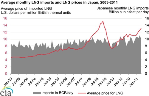
Overall, imports of LNG in Japan have been trending up since 2003. As of April 2011, Japan's total LNG imports accounted for more than 10 BCF per day (see gray area in Figure 6.5) of natural gas supply, most of which are used for power generation. The average price paid for LNG in Japan in 2011 exceeds $13 per million British thermal units (BTU), or about three times the price of natural gas at the Henry Hub in the United States. The price for LNG (light gray line on Figure 6.5) had peaked at $15 per million BTU in 2008, and then fallen to $7 per million BTU in 2009. Since then, the price has been trending back up and now stands at the current $13 per million BTU due to the increased demand in Japan.
Qatar, the largest LNG producer, exported 1800 BCF of LNG in 2009 (5 BCF per day), about 20% of the total global trade based on an analysis in CIA’s recently released Qatar Country Analysis Brief. Its annual LNG exports are equivalent to 8% of U.S. annual marketed natural gas production. Qatar has 14% (894 trillion cubic feet (TCF)) of the world's estimated proved natural gas reserves. It began exporting LNG in 1997 and increased exports to current levels in less than 15 years. Japan, South Korea, and India accounted for 57% of Qatari LNG exports in 2009. European markets including Belgium, the United Kingdom, and Spain imported an additional 33% of Qatari LNG in 2009. North American LNG imports have been relatively low.
In 2010, Qatar exported an estimated 46 BCF of LNG directly to the United States (11% of total U.S. LNG imports) and also exported an estimated 74 BCF to the Canaport LNG terminal in Nova Scotia, Canada, most of which served as supply for New England. Very large investments in infrastructure underpin Qatar's LNG export growth. It has 13 operating LNG trains (liquefaction and purification facilities) with a total LNG capacity of 3400 BCF per year. Five of these trains were added in 2009 and 2010. The most recent addition started commercial service in November 2010 and has an annual production capacity of 380 BCF per year, currently the largest-capacity production train in existence.
Natural Gas Production in the United States
The U.S. natural gas production history was discussed briefly in Chapter 5 and illustrated with production plots in Figures 5.13 and 5.14. U.S. gas production peaked in 1973 at 60 BCF per day before declining to 44 BCF per day in 1986. Since that time, the production has been increasing again and in 2010 the United States had exceeded the 1973 peak and now stands at 63 BCF per day (this only counts the dry gas produced and marketed). Moreover, on the back side of the production curve, the production rate has not followed the bell-shaped curve forecast by Hubbert’s peak oil theory. Gas prices (discussed later) also increased sharply after the production peak of 1973. After this time, the shortfall in demand was partly met by imports from Canada and some limited LNG imports from Trinidad and Qatar. This is shown in Figure 6.6.
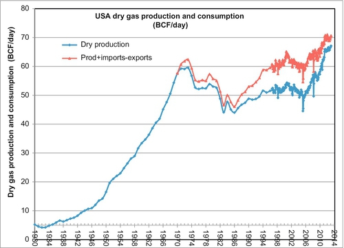
The big increase in production since 1986 has been due to coal-bed methane gas, tight gas, and shale gas. This type of gas is now known collectively as unconventional gas and it accounts for the majority of the current U.S. gas supply. Note that in Figure 6.6 it also shows that natural gas imports also started expanding in 1986 when unconventional gas began its expansion to produce a rapid increase in the natural gas supply in the United States. The steepest increase in the production of gas began in 2006 when the Barnett shale in Texas became economic due to horizontal drilling and multizone fracture stimulation techniques. This also allowed many other shale gas areas to be developed in a similar manner.
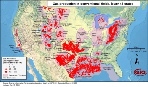
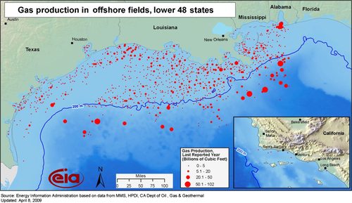
The location of conventional gas fields in the lower 48 states is shown in Figure 6.7. Conventional fields have relatively high porosity and permeability, and the fields are usually developed using vertical wells. Up until 1986, all U.S. gas production came from these types of fields and they still produce a considerable amount of gas. This includes gas produced from offshore fields as shown in Figure 6.8. Most of the offshore production comes from the Gulf of Mexico.
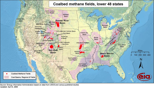
Beginning in 1986, gas began to be produced in significant quantities from various coal-bed methane fields shown in Figure 6.9. Many types of coal have significant quantities of methane adsorbed onto the surface of the coal, which is the bane of coal miners. The methane is maintained on the surface of the coal by pressure. When the pressure is released, the gas desorbs from the coal and can flow through the coal mine or into a well. This can cause underground explosions and asphyxiation of underground miners. It was natural for gas producers to drill wells into coal seams and attempt to produce the gas through vertical wells. It took a lot of experimentation before they could get the gas to flow at commercial rates. Fracture stimulation of the coal bed is usually necessary before the well can become commercial. This technique is discussed in more detail in the next section because it is a vital technique that is common to all unconventional gas.
Coal-bed methane wells were at first quite unproductive. The wells flowed at very low rates. Even with fracture stimulation and under-reaming of the well-bore, the rates were relatively low—less than 1 million cubic feet of gas per day. Conventional gas wells tend to be much higher than that. A second problem was that many coal-bed wells produce a lot of water before any gas starts desorbing from the coal. Producers might typically spend 1 year dewatering the wells before they start producing much gas. This affects the economics significantly. Fortunately, most of the coal seams can be accessed with shallow wells which are cheap to drill and bring into production.
The largest coal-bed methane area has been the San Juan Basin field in northwest New Mexico and southern Colorado. This field, however, has become somewhat depleted and its production is now declining. At its height, the San Juan Basin field was producing about 4 BCF per day, but it is now making about 2 BCF per day, split between New Mexico and Colorado. The largest current coal-bed methane producing state is Wyoming anchored by the Powder River Basin Field, which is currently producing about 1.5 BCD per day; however, it too has begun its decline. Overall, while coal-bed methane is still contributing a robust 5 BCF per day to the U.S. natural gas supply, it is likely to be a decreasing supply source in the future. However, new sources of coal-bed methane are being developed in other countries, such as Australia, China and Russia. In Australia it is called coal seam gas and large supplies of this gas are being developed in the northeast state of Queensland. Most of this gas is being converted to LNG for the export market.
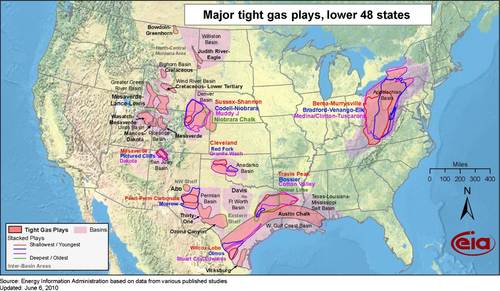
Another major source of unconventional gas in the United States is what has come to be called ‘tight gas’ Figure 6.10 shows the location of the tight gas plays in the United States. There are many of these plays involving a lot of gas. They received a large boost from the success of the Lance and Mesaverde formations in the Jonah and Pinedale fields in Wyoming, starting about 1990. Gas was initially discovered in the Pinedale Anticline in 1955, but was not successfully produced until modern drilling and hydraulic fracturing techniques were developed. The Pinedale Anticline is located within Sublette County, Wyoming, on a narrow, diagonal strip of land that stretches from just outside the Pinedale town limits running along U.S. Hwy 191 for about 30 miles southeast towards Rock Springs. While it is a large narrow anticline, the gas bearing formations are very tight. This means that the permeability of the reservoir rock containing the gas is very low (about 1-10 micro-darcies), and the gas cannot flow out of the rock at fast enough rates to be commercial. When you spend $5 million to drill and complete the well, the gas has to flow at rates higher than 1 million cubic feet of gas per day (depending on the gas price) before you start to get a return on your investment. The early Pinedale wells were flowing at less than one tenth of that rate.
In 1979, the Davis Oil Company drilled a couple of wells on a graben next to the Pinedale Anticline and produced gas from the Lance formation at low to moderate rates; however, they did not consider the rates encouraging enough to continue the exploration. The field was given the name Jonah field but it was not considered commercial. In 1990, Davis sold their wells to a small local company called McMurry Oil Company, led by an entrepreneur called Mick McMurry. He had little experience in the oil and gas business but was eager to learn. McMurry drilled a couple of additional wells and found that by fracture stimulation they could get encouraging rates from the wells. They laid some small bore gas lines down to the Opal gas hub and brought their wells into production. They drilled more wells and continued to improve their fracture stimulation techniques and gradually acquired adjoining leases around the Jonah field and the Pinedale Anticline. Eventually, they were able to prove up about 8 TCF of gas at Jonah and 40–50 TCF at Pinedale. These numbers make both these fields giant gas fields and world class by any standards. The tight reservoirs, however, had proven to be technically difficult to drill and stimulate. The reservoir has over 5000 feet of vertical pay interval, but the productive sands are discontinuous and lenticular. There were considerable technical difficulties to overcome, but the result was a major new source of gas for the United States.
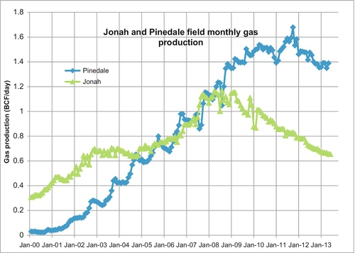
The production data of the two fields is shown in Figure 6.11. In 2007, the combined production surpassed 2 BCF per day and they continue to be produced at these rates. Jonah’s production has been declining since 2008, but this is due to a lack of drilling in the field because of low gas prices. McMurry eventually sold its operating interests in the fields, and it is now produced by a group of companies led by EnCana, Shell, Questar, and Ultra. McMurry’s success opened up many tight gas bearing formations around the country, as shown in Figure 6.10. There is an estimated 500 TCF that will be eventually produced from these “tight” formations.
Meanwhile, another tight gas play was independently developing in Texas in the Barnett shale around Fort Worth and areas to the west. The pioneer here was George Mitchell and his company, Mitchell Energy Company. Mitchell has had gas-producing leases in the Fort Worth Basin since the 1950s, but he began to test wells in the Barnett shale around 1980. He was unable to make any commercial wells in the formation for the first 20 years of work. The Barnett shale was even tighter than the Lance formation that McMurry was drilling in Wyoming. The permeability of the Barnett is measured in nano-darcies and nothing like that had ever been successfully produced. Mitchell tried many different methods of stimulating the Barnett shale over a long period of time to try and coax commercial quantities of gas from the formation. Eventually, he was able to make it economic by drilling horizontal wells through the formation followed by many large fracture stimulation jobs using water-based fluids.
The average Barnett well now makes more than 2 million cubic feet of gas per day and can recover more than 5 BCF of gas per well. Mitchell eventually sold his company for about $3.5 billion. George Mitchell initiated a revolution in natural gas supply in the United States because a huge amount of gas is trapped in similar formations around the country. Eventually this technology will be exported to the rest of the world and huge new gas reserves will be produced in many other countries. It seems like the United States always leads the way on these sorts of technical innovations. This is motivated by their continuing need for energy resources to fuel their economy and maintain their culture.
Figure 6.12 shows the location of the current shale plays in the lower 48 states of the United States. Besides the Barnett, the other hot shale gas plays have been: the Haynesville in northern Louisiana; the Fayetteville in Arkansas; the Woodford in Oklahoma; the Eagle Ford in Texas; and, the Marcellus in West Virginia, western Pennsylvania, southern New York, and eastern Ohio. The biggest of these plays is the Marcellus shale, and it has barely begun to be developed. Figure 6.13 shows its location. Just like McMurry, Mitchell’s success in the Barnett shale has opened up production in many other formations around the United States and Canada.
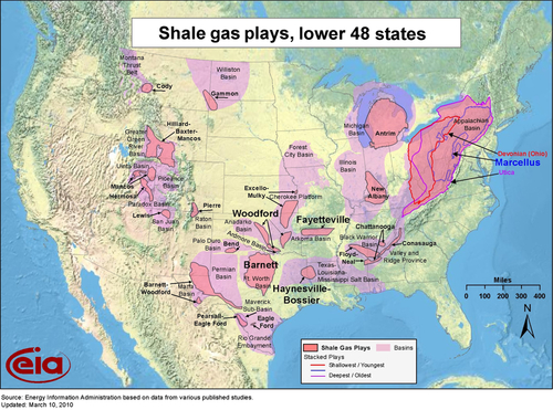
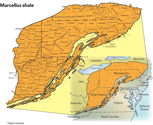
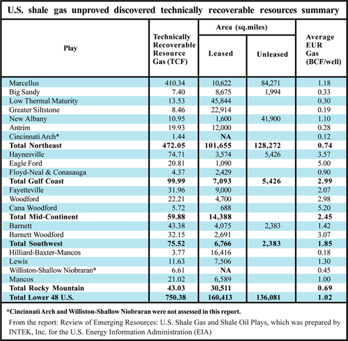
Figure 6.14 shows a table from a recent (2011) report on shale gas reserves prepared by INTEK for the U.S. Energy Information Administration (EIA). It has identified 750 TCF of unproven but technically recoverable reserves in these shale plays. The reserves are unproven because wells have not yet been drilled to prove the gas is actually there under each acre of earth where the formation is known to exist. At the same time, the numbers in Figure 6.14 may be conservative because it only shows 410 TCF of gas for the Marcellus and 43 BCF for the Barnett. In other reports, estimates have been as high as 1500 TCF for the Marcellus and 150 BCF for the Barnett. These reports may not be as reliable as the INTEK-EIA report but they are certainly more optimistic. Compare that to the listed proved reserves of gas for the entire United States of 162 TCF in 1993 and the current (2010) EIA listed proved reserves of gas of 272 TCF. The largest proved gas reserves in U.S. history were 293 TCF in 1967. These new reserves of gas are massive and are causing a paradigm shift in the supply of natural gas in the United States, which has driven the price back down to much cheaper levels.
Natural Gas Storage
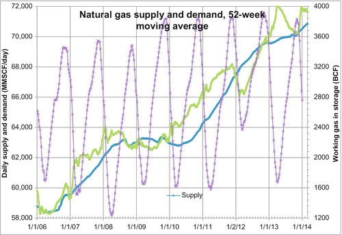
Figure 6.6 gives a picture of the annual and monthly supply of natural gas in the United States, but it does not tell the full story. The demand for natural gas is seasonal, having high demand for space heating in the winter and lower demand in the spring, fall and summer. Summer demand has been increasing because more gas is now used to generate electricity for air conditioning in the summer. Nevertheless, the highest demand for natural gas occurs in the wintertime.
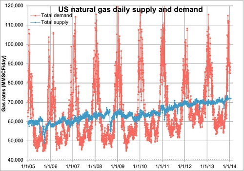
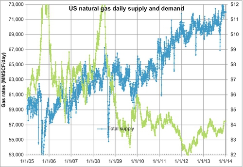
Figure 6.15 shows the daily supply and demand for natural gas from January 2005 to August 2011. The light gray line is the demand curve and the gray line is the supply curve. There are clearly large seasonal variations in demand. In order to reduce the size of pipelines and also to provide a security of supply, it is more efficient to produce the gas at the same rate all year, store it close to the market (the end user) during the spring, summer and fall, and produce it from both the storage facility and the gas fields for use in the winter. For this purpose, gas is stored in underground reservoirs for when the need arises. There are several important reasons for storing gas in these underground facilities:
• The size of the pipelines transporting the gas are reduced
• It allows the gas fields to be produced at a constant rate
• It provides a security of supply when interruptions occur, and
• It allows for trading and balancing of supply from different sources.
The fourth item bears some explanation. In the past, U.S. gas contracts were often written with “take or pay” provisions. This meant that, if the utilities buying the gas did not need all the gas in the contract, it had to produce and store the gas in the storage reservoirs or pay penalties. Take or pay contracts are less common in today’s market, but with the deregulation of the U.S. gas industry that resulted from the FERC Order No. 636 (issued on April 8, 1992), new reasons for storing gas became evident. As the price became more volatile, gas buyers tried to buy the gas at low prices and store it for later use or resale at higher prices. In this environment, the demand for gas storage facilities increased. Under current circumstances, the gas does not need to be stored close to the end-user but can be stored anywhere along the pipeline, particularly near pipeline interchanges.
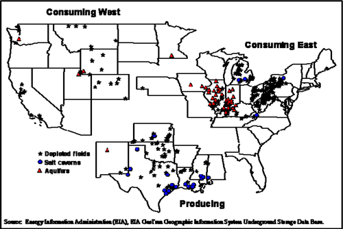
The operators of underground storage facilities are usually pipeline companies and local distribution companies, but there are some independent storage service providers. There are about 80 companies that currently operate the nearly 400 underground storage facilities in the lower 48 states. The location of these storage facilities are shown in Figure 6.16. There it can be seen that there are three types of reservoirs used to store gas: depleted oil and gas fields; salt caverns; and, salt-water aquifers. If a storage facility serves interstate commerce, it is subject to the jurisdiction of the FERC; otherwise, it is regulated by the state authority.
Operators of storage facilities are not usually the owners of the gas held in storage. Most working gas held in storage facilities is held under lease with traders, gas distribution companies, and even end users who buy the gas before they need to use it. The United States has the most efficient gas storage system in the world. Figure 6.17 shows the total amount of gas held in storage over the past 6.5 years. As can be seen, the total gas in storage at any one time is divided up into the base gas and the working gas. The base gas (also called the cushion gas) is the volume of gas intended as permanent inventory in a storage reservoir needed to maintain adequate pressure and flow rates throughout the winter withdrawal season. Working gas is the volume of gas in the reservoir above the level of base gas that is available to be withdrawn in the winter. Working gas capacity is equal to the total gas storage capacity minus the base gas. The specification of what is base gas and what is working gas is somewhat arbitrary in that during a crisis of supply some of the base gas could be withdrawn to satisfy an emergency. Usually, the base gas is left in the storage reservoir permanently and is never withdrawn. The working gas is injected into the storage reservoirs in the spring, summer and fall and produced again in the wintertime. This provides a tremendous back-up and security of supply to the U.S. gas consumer and keeps the whole supply chain moving along in a most reliable manner.
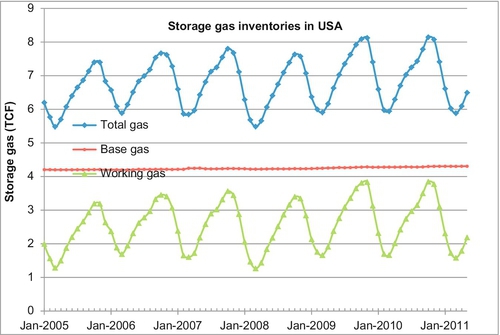
In Figure 6.17, it can be seen that the base gas remains relatively constant at about 4.3 TCF. The working gas varies from about 1.25 TCF up to 3.8 TCF. The total gas in storage varies from 5.55 TCF to 8.1 TCF. There is always more than 5.5 TCF gas in storage, even at the end of the winter season when the storage gas is relatively depleted.
To illustrate the importance of gas storage, one only has to look at the effects a single accident had in a natural gas facility in the Australian state of Victoria in September 1998. The largest city in the state of Victoria is Melbourne, a bustling city of 4 million people—the second largest in Australia. The city of Melbourne and the entire state of Victoria is supplied with natural gas from the offshore oil and gas fields in the Bass Strait, south of the state, and operated by a subsidiary of Exxon. The gas from the fields is processed at three gas plants at Longford (near the city of Sale) and then is piped to Melbourne and to other cities further afield. Natural gas is the primary heating source for 80% of Victorian households, 50% of the commercial enterprises and 25% of industry.
On Friday, September 25, 1998, a vessel ruptured at one of the gas plants leading to several explosions and fires. These fires and leaks continued at the plant until the last fires were extinguished 2 days later on Sunday, September 27. The winter months in Australia are June, July, and August. Even though the winters in Melbourne are not as fierce as in North America, the weather was still somewhat cool and the loss of the gas supply left a lot of people without heat.
As a result of the fires and explosions, all three gas plants were shut down. As Victoria is not connected to any gas storage facilities, supplies of gas to all domestic, commercial and industrial consumers in metropolitan Melbourne and in several areas beyond were shut down. Most Victorian gas consumers were left without gas for 19 days. The accident and subsequent loss of supply is considered to have been one of Victoria’s worst economic disasters. It is estimated that 1.5 million households and 90,000 businesses were affected. In addition to directly affecting the daily lives of 4.5 million people for almost 3 weeks, the estimated cost of the accident to the Victorian economy was put at $1.5 billion. Industrial sectors particularly affected included the car industry, plastics production, food and drink manufacturers and the hospitality sector. Tens of thousands of workers were temporarily unemployed and several manufacturing industries were forced to shut down for a month. The disaster spawned the largest class action suit in Australian legal history, with 10,000 litigants signed on. Other impacts included temporarily curtailed production of some basic consumables including bread, milk, and other dairy products. Supply lines of basic consumables had to be brought in from out-of-state sources to overcome local shortfalls. This disruption would not have occurred if there was a large gas storage facility located near Melbourne. Gas could be withdrawn from the storage facility until the regular supply resumed.
The Price of Gas
In Figure 5.14 of Chapter 5, it was shown that the average annual price of natural gas in USA had been driven up by the reduced supply of natural gas after its production peaked in 1973. In recent years, the price of natural gas has been quite volatile. As with any commodity, the price of gas is governed by supply and demand. When demand outstrips supply, the price rises; when the supply outstrips demand, the price falls. Due to the seasonal variations in demand, it is not a simple task to measure when supply and demand are out of balance. There are also the follow-up questions as to the factors that affect supply and demand. Figure 6.15 showed that demand in particular is always rising and falling relative to supply and in the last section it was shown that the industry has learned to balance these variations using natural gas storage. These factors can mask a supply/demand imbalance. The price of gas in the United States is usually quoted in dollars per million BTU, abbreviated $/MMBTU. The primary source of the price data is the New York Mercantile Exchange, abbreviated NYMEX.
Gas was previously sold under long-term fixed price contracts. This was beneficial to both buyer and seller because both knew exactly what price was being paid for the gas over the entire life of the contract. These contracts were also necessary to finance field development. Bankers would not lend money on the development of a gas field unless the long-term contract was in place, which assured the banker that money would be there to repay the loan. These contracts had take or pay provisions whereby the buyer (a large well financed utility or a large industrial user) would be required to pay for the gas whether they took delivery of it or not. While much of the risk lay with the buyers, they had a fixed price that removed the risk of cost increases. Over time these types of contracts fell out of favor because, after spot prices began to rise in the late 1970s, gas producers found that being locked into long-term low price contracts removed any upside potential for their product. Moreover, when the industry was deregulated and made more open by FERC Order 636 in 1992, it created the conditions that allowed for contracts and sales at the market price for gas.
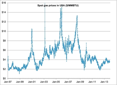
Figure 6.18 shows the daily spot price for natural gas since January 1, 1997. The spot price is the price paid for daily deliveries of gas at the prevailing price. The data shows that the spot price can spike rapidly when shortages develop. The majority of gas is not actually sold at the spot price or in long-term fixed price contracts. The majority of gas is now sold under futures contracts. A futures contract is a promise to deliver gas during a certain month at a particular price. The futures price for four forward months is shown in Figure 6.19. These show the same volatilities and price spikes as the spot price trends; however, the spikes are not quite as severe. On February 25, 2003, for example, the spot price peaked at $18.48 per MMBTU from a price of $5.88 per MMBTU on February 14. By March 5, 2003 the price was back down to $7.80 per MMBTU, and it continued declining from there. This brief spike was caused by a reduction in supply and an increase in demand during a winter blast of cold weather. The forward months futures prices also spiked, but at $9.58 for the one-month futures contract and $6.58 for the two-month futures contract. The three-month and four-month contract did not react at all because this was a short-term temporary situation.
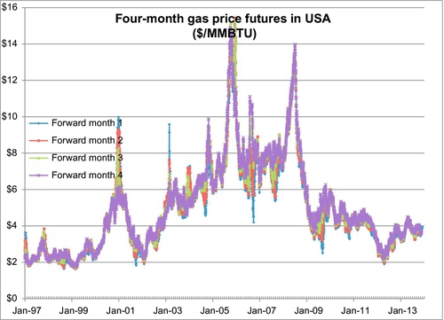
Examination of Figure 6.19 indicates that the four forward months futures prices usually follow each other across long-term trends. When the one-month price increases, the two-, three-, and four-month future prices also increase, and vice versa. While this is often the case, it is not always true, as will be seen later.
The question remains as to what exactly causes these spikes. Why does the price run up and what causes it to return to prespike prices? Figure 6.20 shows the spike that occurred in the winter of December 2000 to January 2001. A severely cold winter caused a larger than usual demand for gas for heating, and the price shot up. There was no real shortage of gas because the extra demand was filled from storage gas. Traders, however, recognized that when a larger than usual supply comes from storage gas, this gas must eventually be replaced and more gas must eventually be produced to replace the gas being used by the cold winter. This pushes the price up.
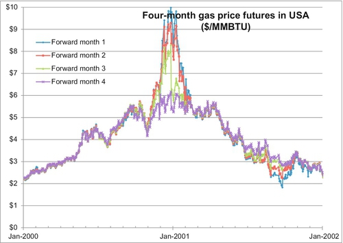
Throughout the year 2000, the price of gas had been rising gradually and the four future month’s prices tracked each other very closely. The market was saying that if the price is rising now, these conditions will still exist in four months and the price for four months in the future will also rise by the same amount. When the price spike came in December 2000, the four-month price separated from the one-month price because the market perceived that the conditions pushing the price up in December may still exist in January but probably would be over by April when the cold winter had receded. Indeed by April 2001, the price of gas was declining and the four future month’s prices declined in lockstep with one another. By September 2001, the future months were separating again. While low demand in September may justify the price continuing to fall, the four-month future price was for December 2001 when another cold winter might be looming. There were no price spikes in the winters of January 2000 or January 2002 because these winter were normal and did not result in any demand for gas above and beyond the normal high winter demand.
In September 2005, another huge price spike occurred, but this one was not caused by unusually cold winter weather. To illustrate what happened, Figure 6.21 shows the one-month forward price along with the daily supply curve from Bentek’s daily production data. In September 2006 two huge hurricanes tore through the Gulf of Mexico: Hurricane Katrina and Hurricane Rita. In addition to destroying New Orleans, they also shut down most of the oil and gas production in the Gulf of Mexico for several months. The total U.S. gas supply dropped from about 60 BCF per day to about 52 BCF per day. This created a temporary shortage of gas for about 2 months. When the offshore platforms returned to production, the price returned to normal levels. This was a price spike caused by a temporary supply interruption.
A similar supply interruption was caused by two more Gulf of Mexico hurricanes in September 2008 when Hurricanes Gustav and Ike shut in another 10 BCF per day. This time the supply interruption did not cause a price spike and the reason is rather interesting. In the summer of 2008, a gas price spike developed due to rising demand. The robust economy of 2007 and early 2008 produced rising gas demand, which caused the price of gas to run up to $14 per MMBTU. These high prices then caused the demand to soften and the price began to decrease again. By September 2008, the world financial crisis—precipitated by bad subprime loan defaults—suddenly hit the market and the price of gas continued to decrease rapidly. When the hurricanes hit at the same time as the financial crisis, the market ignored the supply interruption because there was a strong perception that demand was going to be greatly decreased by a weakening world economy. The supply disruption had no effect on the gas price.
To keep track of the balance between supply and demand, traders primarily use the weekly gas storage numbers released by the EIA of the U.S. government. These can be just as difficult to interpret because they also change with the season. A more effective method is to plot the moving average of the supply and demand. If 52-week or 1-year moving averages of supply and demand are compared, you can see over the past year if the supply or the demand has been higher and whether the price should be increased or decreased. The peaks and valleys of the working gas in storage are useful information, but these only occur twice per year. Each week (on Thursdays at 10:30 am EST) when the storage data is released, traders compare the storage levels to the same week of the previous 5 years and try to adjust the price according to their interpretation of the data.
Figure 6.22 shows the 52-week moving average of supply and demand along with the weekly working gas in storage values. In 2007 and early 2008, the average demand was rising faster than the average supply. This resulted in the storage gas in early 2008 being reduced to less than 1.5 TCF, its lowest level in many years. This was a signal for the price to be pushed up in the spring and summer of 2008. When the world financial crisis hit in late 2008, demand was indeed scaled back. The storage low of early 2009 was above 1.6 TCF, and the storage high of November 2009 was above 3.8 TCF, its highest value ever. These were signals for the gas price to be pushed down to $2.51 per MMBTU on September 9, 2009, its lowest price since March 2002.
When the Gulf of Mexico production was restored after the damage and devastation caused by Hurricanes Katrina and Rita in September 2005, the supply of gas in the United States received a major boost with the success of the shale gas revolution. The large increases in supply from January 2006 to the present time, seen in Figure 6.21, are due to the Barnett shale production, followed by the Fayetteville in Arkansas, the Woodford in Oklahoma, the Haynesville in northern Louisiana, and more recently by the Eagle Ford in Texas and the Marcellus in Pennsylvania.
The other factor that affects the natural gas supply is the number of gas wells that are being drilled. Most gas wells produce at their highest rate at the beginning of their productive lives. Very soon after a gas well goes on production, its production rate begins to decrease as the pressure in the reservoir decreases. If the industry is not continuously drilling new wells, the gas supply will naturally decrease. Traders watch the drilling rig report to see how many wells are being drilled and put into production. This is an indication of how much the gas production rate will be increasing or decreasing in the future. Most wells that are drilled these days are going to be successful producers so the rig report is a strong indicator of future supply.
State Production and Transportation of Natural Gas in USA
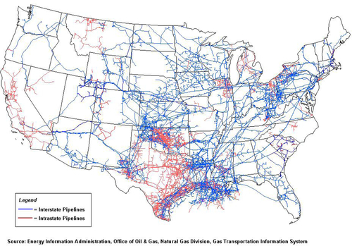
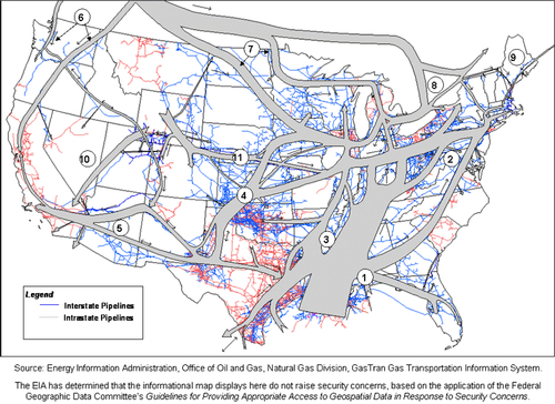
The United States has the most efficient and widespread natural gas pipeline network in the world. As shown in Figure 6.23, the gray lines represent interstate pipelines and the light gray represent intrastate pipelines. This network is continually being revised as production in some locations declines and new fields are brought into production. With the paradigm shift to unconventional gas in the past 5 years, a large reorientation of the pipeline network has occurred. Nevertheless, with such a dense and ubiquitous network in place, it is relatively easy and rapid to respond to new production in most places. Figure 6.23 does not give an accurate picture of the amount of gas moving in the pipelines because the diameter of the pipelines is not shown. The larger the diameter, the greater the amount of gas that can flow through the pipeline for a given pressure gradient in the pipeline. Figure 6.24 shows the corridors where the gas is currently flowing. The width of the corridors indicates the volume of gas flowing through the pipeline network. Further details about the directions and volumes of flows can be found on the EIA website.
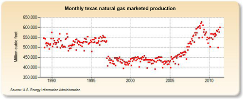
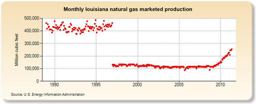
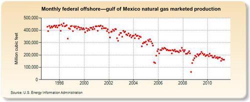
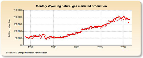
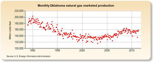
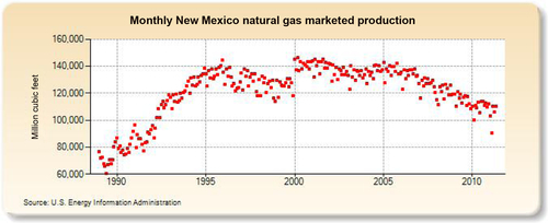
The largest gas-producing state is Texas (see production in Figure 6.25), and this is reflected in the network of pipelines that crisscross the state including the offshore Gulf of Mexico area, where a great deal of gas is produced. The second-largest gas-producing state is Louisiana, which overtook Wyoming for second place in 2010 due to large increases in its shale gas production from the Haynesville formation. Its production history is shown in Figure 6.26. The Federal Offshore Gulf of Mexico natural gas production, which has been steadily declining in recent years, is shown in Figure 6.27. The Federal Offshore Gulf of Mexico production has only been taken into account since 1997. Prior to that, the offshore Gulf of Mexico production was counted in state figures. That is why Texas and Louisiana show a decrease in production in 1997. The third-, fourth-, and fifth-largest gas-producing states are Wyoming, Oklahoma, and New Mexico, whose production volumes are shown in Figures 6.28–6.30, respectively.
Fracture Stimulation Techniques
All of the unconventional gas now being produced in the United States has been made economic by the hydraulic fracturing process (commonly known as “fracking”), in which water, chemicals and proppant materials are pumped into the well to release the gas trapped in low permeability formations by creating fractures in the rock and allowing natural gas to flow from the rock into the well. This process is illustrated in Figure 6.31.
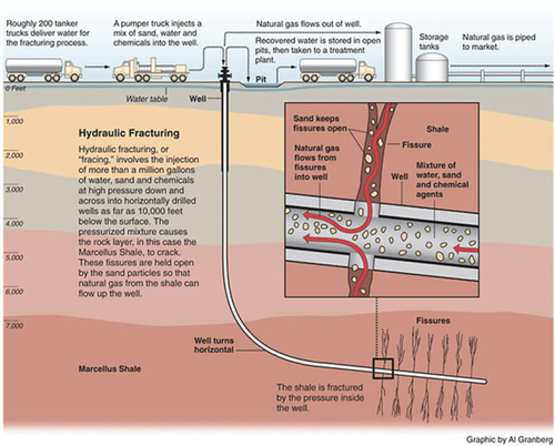
After the water-based fluid creates the fracture, the proppant is pumped down the well transported by a carrier fluid. The purpose of the proppant is to prop open the fracture so that it does not close up again, which allows the gas to flow out of the formation through the fracture. Most commonly the proppant is sand, which is sometimes coated with resin. The proppant can also be aluminum bauxite or special ceramics, which are mainly used when the weight of the overburden rock is very high and creates high stresses. When the overburden stress is too high, the regular sand particles get crushed in the fracture and the fracture closes up. Ceramic proppants are more expensive than sand, so they are only used when sand will not do the job. The carrier fluid used to transport the proppant down into the fracture is often borate-based cross-linked gel polymers. These polymers are used because they can carry a lot of proppant out into the formation. The more proppant placed in the fracture, the better it works. After a certain period of exposure to the higher temperatures in the formation, the chemical bonds in the cross-linked gel polymer break down and the polymer becomes more fluid, which allows it to flow back out of the formation, leaving the proppant behind. Cross-linked gel polymers are widely used as carrier fluids in hydro-fracturing operations.
Most of the shale gas-fracturing operations use a so-called slick-water fracture fluid. It is called slick-water because gel polymers are not used, but chemicals are added to the water-based fracturing fluids to reduce the water’s viscosity to make it flow more readily. Slick water cannot carry proppant as effectively as the gels, but it seems to be able to create a broader network of induced fractures in the shale, which makes the shale more productive. Slick water fracks are also cheaper as well as being more effective in some shale formations.
One of the environmental concerns about fracturing operations is that some of the chemicals used can contaminate freshwater formations. This should not happen because the shale formations are usually widely separated from the freshwater aquifers by thousands of feet of rock. Accidents can occur, however, and fracturing fluid containing chemicals could be spilled on the ground and then washed into aquifer recharge areas. As of the current moment, there have not been any such incidents and there have not been any water supplies contaminated by fracturing fluids. Despite this, regulatory authorities are now requiring fracturing service companies to identify the chemicals being used in their operations so that if water wells do end up contaminated, the contamination can be traced.
Liquid Transportation Fuels from Natural Gas
Natural gas can be used to manufacture petrochemicals such as methanol, ammonia, fertilizer, and polymers; however, these are relatively small users of the gas reserves with limited markets. Liquid fuels represent a much larger market. Moreover, they can be moved in existing pipelines or product tankers and even blended with existing crude oil or product streams. No special contractual arrangements are required for their sale in most markets.
The technology to convert gas to liquids (GTL) is well known, and new technology is being developed and applied on a regular basis. The technology is scalable, allowing design optimization and application to smaller gas deposits. The key influences on their competitiveness are the cost of capital, operating costs of the plant, feedstock gas costs and the ability to achieve high utilization rates in production. As a generalization, however, GTL has not been competitive against conventional oil production unless the gas has a low opportunity value and is not readily transported. When oil is selling for close to $100 per barrel, the economics become much more attractive, as will be seen later.
GTL not only adds value, but is capable of producing products that could be sold or blended into refinery stock as superior products with fewer pollutants for which there is growing demand. Reflecting GTL’s origins as a gas, GTL processes produce diesel fuel with an energy density comparable to conventional diesel, but with a higher cetane number permitting a superior performance engine design. Another “problem” emission associated with diesel fuel is particulate matter, which is composed of unburnt carbon and aromatics and compounds of sulfur. Fine particulates are associated with respiratory problems, while certain complex aromatics have been found to be carcinogenic. Low sulfur content leads to significant reductions in particulate matter that is generated during combustion, and the low aromatic content reduces the toxicity of the particulate matter. This has resulted in a worldwide trend towards the reduction of sulfur and aromatics in fuel.
It is technically feasible to synthesize almost any hydrocarbon from any other. In the past five decades, several processes have been developed to synthesize liquid hydrocarbons from natural gas. Indirect conversion to liquids can be carried out via Fischer-Tropsch (F-T) synthesis or via methanol. The discovery of F-T chemistry in Germany dates back to the 1920s, and its development has been for strategic rather than economic reasons, as in Germany during World War II and in South Africa during the apartheid era. Mobil developed the “M-gasoline” process to make gasoline from methanol, and this was implemented in 1985 in a large integrated methanol-to-gasoline (MTG) plant in New Zealand. The New Zealand plant was a technical success, but produced gasoline at costs above $30 per barrel. This was higher than the cost of refining gasoline from crude oil in the 1980's and 1990's. The plant was eventually converted to methanol-only production.
The first step in the GTL process is to convert the natural gas to syngas (which consists of hydrogen and carbon monoxide) by partial oxidation, steam reforming or a combination of the two processes. The key variable is the hydrogen to carbon monoxide ratio with a 2:1 ratio recommended for F-T synthesis. Steam reforming is carried out in a fired heater with catalyst-filled tubes that produce a syngas with at least 5:1 hydrogen to carbon monoxide ratio. To adjust the ratio, hydrogen can be removed by a membrane or pressure swing adsorption system. This process is widely used if the surplus hydrogen is used in a petroleum refinery or for the manufacture of ammonia in an adjoining plant. The partial oxidation route provides the desired 2:1 H:C ratio and is the preferred route in isolation of other needs.
Conversion of the syngas to liquid hydrocarbon is a chain growth reaction of carbon monoxide and hydrogen on the surface of a heterogeneous catalyst. The catalyst is either iron- or cobalt-based, and the reaction is highly exothermic. The temperature, pressure and catalyst determine whether light or heavy products are produced. For example, at 330 °C mostly gasoline and olefins are produced whereas at 180-250 °C mostly diesel and waxes are produced. Similar technologies are used to make liquid transportation fuels from coal, and more details on these technologies are given in Chapter 13. It is slightly more difficult to make syngas from coal, but once created, the syngas is converted into gasoline and diesel fuels using the F-T process in exactly the same manner.
The South African company, Sasol, is a technology supplier that was originally formed to provide synthetic petroleum products to South Africa during the apartheid era. The firm has built a series of F-T coal-to-oil plants and is one of the world's most experienced synthetic fuel organizations. It is now marketing a natural GTL technology. It has developed the world's largest synthetic fuel project, the Mossgas complex at Mossel Bay in South Africa. This project was commissioned in 1993 and produces 25,000 barrels per day. To increase the proportion of higher-molecular-weight hydrocarbons, Sasol has modified its Arge reactor to operate at higher pressures. It has commercialized four reactor types, with the slurry phase distillate process being the most recent. Its products are more olefinic than those from the fixed bed reactors and are hydrogenated to straight chain paraffins. Its slurry phase distillate converts natural gas into liquid fuels, most notably superior-quality diesel, using technology developed from the conventional Arge tubular fixed-bed reactor technology. The resultant diesel is suitable as a premium blending component for standard diesel grades from conventional crude oil refineries. Blended with lower grade diesels, it makes it easier to comply with the stringent specifications being set for transport fuels in North America and Europe.
Its other technology uses the Sasol Advanced Synthol (SAS) reactor to produce mainly light olefins and gasoline fractions. Sasol has developed high performance cobalt-based and iron-based catalysts for these processes. The company claims a single module of the Sasol slurry phase distillate plant converts 100 million cubic feet per day (110 TJ per day) of natural gas into 10,000 barrels per day of liquid transport fuels and can be built at a capital cost of about US$250 million. This cost equates to a cost per daily barrel of capacity of about US$25,000, including utilities, off-site facilities, and infrastructure units. If priced at $5 per MMBTU, the gas amounts to a feedstock cost of US$50 per barrel of product. The fixed and variable operating costs (including labor, maintenance, and catalyst) are estimated at a further US$5 per barrel of product, thereby resulting in a direct cash cost of production of about US$55 per barrel (excluding depreciation). Most of this cost is for the gas feedstock.
In June 1999, Chevron and Sasol agreed to an alliance to create ventures using Sasol's F-T technology. The two companies have conducted a feasibility study to build a GTL plant in Nigeria that was to begin operating in 2013. This joint venture (Chevron and Sasol) has also partnered with the Nigerian National Petroleum Corporation to build the GTL plant, which is expected to convert 325 million cubic feet of natural gas per day into 33,000 barrels of liquids, principally synthetic diesel. When completed, the plant is expected to export the diesel fuel product to Europe.
Shell has carried out research and development (R&D) since the late 1940s on the conversion of natural gas, leading to the development of the Shell middle distillate synthesis (SMDS) route—a modified F-T process. SMDS focuses on maximizing yields of middle distillates, notably kerosene and diesel and bunker fuel. Shell built a 12,000 barrel per day GTL plant in 1993 in Bintulu, Malaysia. The process consists of three steps: the production of syngas with a H2:CO ratio of 2:1; syngas conversion to high-molecular-weight hydrocarbons via F-T using a high performance catalyst; and hydro-cracking and hydro-isomerization to maximize the middle distillate yield. Shell is investing US$6 billion in GTL over 10 years with four plants. It announced in October 2000 that there was an agreement with the Egyptian government to build a 75,000 barrel per day facility in Egypt and a similar plant to be built in Trinidad & Tobago. In April 2001, it announced interest for plants in Australia, Argentina and Malaysia at 75,000 barrels per day costing US$1.6 billion.
Exxon has developed a commercial F-T system from natural gas feedstock. Exxon claims its slurry design reactor and proprietary catalyst systems result in high productivity and selectivity along with significant economy of scale benefits. Exxon employs a three-step process: fluid bed synthesis gas generation by catalytic partial oxidation; slurry phase F-T synthesis; and fixed bed product upgrade by hydro-isomerization. The process can be adjusted to produce a range of products. More recently, Exxon has developed a new chemical method based on the F-T process to synthesize diesel fuel from natural gas. Exxon claims that better catalysts and improved oxygen-extraction technologies have reduced the capital cost of the process and is actively marketing the process internationally. Made from gas, the high-molecular-weight liquid GTL products can be hydro-cracked in a simple low-pressure process to produce naphtha, kerosene, and diesel that is virtually free of sulfur and aromatics. These derivative fuels are therefore potentially more valuable, notably in the United States, Europe, and Japan because of their high environmental standards.
The Syntroleum Corporation in the United States is marketing an alternative natural-gas-to-diesel technology based on the F-T process. It claims to be competitive with a lower capital cost due to the redesign of the reactor. Instead of oxygen, an air-based auto-thermal reforming process is used for synthesis gas preparation to eliminate the capital expense of an air separation plant. This type of catalyst results in high yield. It claims to be able to produce synthetic crude at around $50 per barrel. The syncrude can be further subjected to hydro-cracking and fractionation to produce a diesel/naphtha/kerosene range at the user’s discretion. The company indicates its process has a capital cost of around $13,000 per daily barrel of diesel for a 25,000 barrel per day facility and an operating cost between $3.50 and $5.70 per barrel.
The thermal efficiency of the Syntroleum process is reported to be about 60%, implying a requirement of about 90 million cubic feet (85 TJ) per day of dry gas for a 25,000 barrel per day facility costing $350 million. These figures indicate a unit cost of less than $50 per barrel ($8 per GJ) of diesel fuel. The Syntroleum Corporation now also licenses its proprietary process for converting natural gas into other synthetic crude oils and transportation fuels. In February 2000, Syntroleum Corporation revealed its plans to construct a 10,000 barrel per day (requiring 130 TJ per day or 800,000 tons per year of gas) GTL plant for the state of Western Australia. This project did not get built. The project planned to produce synthetic specialty lubricating oils, naphtha, normal paraffin, and drilling fluids and was estimated to cost US$500 million, generating sales of around US$200 million per year.
On August 1, 2011, China Petroleum & Chemical Corporation (Sinopec) and Syntroleum Corporation announced the opening of the Sinopec/Syntroleum Demonstration Facility (SDF) located in Zhenhai, China. It is an 80 barrel per day facility utilizing the Syntroleum-Sinopec F-T technology for the conversion of coal, asphalt and petroleum coke into high-value synthetic petrochemical feedstocks.
Rentech Inc. in Denver, Colorado, has been developing an F-T process using a molten wax slurry reactor and precipitated iron catalyst to convert gasses and solid carbon-bearing material into straight chain hydrocarbon liquids. In their process, long straight chain hydrocarbons are drawn off as liquid heavy wax while the shorter chain hydrocarbons are withdrawn as overhead vapors and condensed to soft wax, diesel fuel, and naphtha. It is promoted as suitable for remote and associated gas fields as well as sub-pipeline quality gas. It currently has a 10 barrel per day demonstration plant operating in Commerce City, Colorado.
There are several methanol-based routes to manufacture gasoline from syngas. The principal one is Mobil’s MTG process based on their ZSM-5 zeolite catalyst, which was commercialized in 1985 in the GTL plant now owned by Methanex in New Zealand. Commercial applications of the MTG process are now anticipating using a fluid bed reactor because of its higher efficiency and lower capital cost.
The use of GTL for chemical and energy production is forecast to advance rapidly with increasing pressure on the energy industry from governments, environmental organizations, and the public to reduce pollution, including the gaseous and particulate emissions traditionally associated with conventional petroleum-fueled and diesel-fueled vehicles. The commercial success of GTL technology has not yet been fully established and returns from GTL projects will depend on projections of market prices for petroleum products and presumed price premiums for the environmental advantages of GTL-produced fuels. Unit production costs will reflect: the cost of the feedstock gas; the capital cost of the plants; marketability of by-products such as heat, water, and other chemicals (e.g., excess hydrogen, nitrogen, or carbon dioxide); the availability of infrastructure; and the quality of the local workforce. Clearly, the feedstock gas cost will have an influence as it may vary widely depending on alternative applications. As one indication, based on current efficiencies, a change in the cost of gas feedstock of $0.50 per million BTU (or per one gigajoule GJ) would shift the synthetic crude oil price by around $5 per barrel. This is predicated on the relationship that the processes require about 10 MMBTU (10.5 GJ) of gas to produce 1 bbl of fuel with variations depending on scale, quality of output and variable production costs traded off against capital costs.
Shell estimates that a GTL plant processing 600 million standard cubic feet (0.7 TJ) of gas per day would cost 60% more than an LNG plant, but the more readily used end-products make GTL cheaper than LNG. According to Shell, a 75,000 barrel per day plant would cost around US$1.6 billion.
Capital costs for GTL projects currently tend to be in a range of double that of refineries, between $20,000 and $30,000 per daily barrel of capacity (compared with refinery costs of $12,000-$14,000 per daily barrel). The cost of GTL-produced fuel could also vary by approximately $1.50 per barrel with a shift of $5000 in capital cost. Estimates of the crude oil prices necessary to allow positive economic returns from a GTL project vary widely, with optimistic estimates ranging as low as $14-$16 per barrel plus fuel costs.
Presently there are only four GTL facilities producing synthetic petroleum liquids at more than a demonstration level: the Mossgas Plant (South Africa), with an output capacity of 23,000 barrels per day; the Shell Bintulu plant in Malaysia at 20,000 barrels per day; and the MTG project in New Zealand, which is now making only methanol. The fourth and largest GTL project is the recently completed Shell GTL plant in Qatar. It uses 1.6 BCF per day of gas to produce about 140,000 barrels per day of liquid fuels. The joint project in Nigeria of Chevron, Sasol and Nigerian National Petroleum Corporation to build a 30,000 barrel per day plant costing $1 billion using the Sasol Slurry Phase Distillate process was expected to begin operations in 2013. The Nigeria project would benefit from the infrastructure already in place for nearby oil and gas production and export facilities.
The Future of Natural Gas
The future for natural gas is very bright, particularly in the United States, which is already the world’s largest producer and consumer of natural gas. With the large deposits of shale gas that have recently been made economic, there are abundant new supplies to be produced. Currently, the United States is producing about 68 BCF per day of total gas, netting 63 BCF per day of marketed dry gas as well as a large amount of condensate and natural gas liquids. This has allowed the United States to reduce its volume of imported oil from a high of 13.4 million barrel per day in August 2006 to the current (in 2014) 5 million barrel per day. The United States has the capacity to double its current gas production to as much as 136 BCF per day and convert the additional gas to electricity or to liquid transportation fuels, displacing much more imported oil in the process. If all of the additional 68 BCF per day of gas was converted into liquid transportation fuels, it would amount to 7 million barrel per day less imported oil. If the gas was used to generate electricity instead and the electricity was used to power electric vehicles, a similar volume of crude oil could be displaced. If the 136 BCF per day were maintained for the next 30 years, it would require reserves of 1500 TCF of gas. There is every expectation that the oil and gas industry can prove up that volume of gas.
In order to increase the gas production rate by 68 BCF per day, about 34,000 new wells would have to be drilled with the assumption that each well would have an average initial rate of 2 million cubic feet per day. After that, an additional 20,000 wells per year would have to be drilled to keep the gas production rate at a constant 136 BCF per day. It would be a significant logistical task to drill that many wells each year, but the oil and gas industry is capable of doing it. Shale gas and tight gas wells are not cheap to drill and the industry would not drill the wells if the gas markets were not developed and a minimum gas price was not certain. An estimate is that a gas price of $5 per MMBTU would be required and at this price the industry could produce transportation fuels for about $70 per barrel. The current (2014) wholesale price for gasoline is $2.85 per gal, which is equivalent to $120 per barrel.
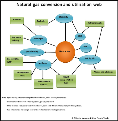
There are many uses for natural gas, which are summarized in Figure 6.32. It is most widely used for space heating, but Figure 6.32 shows that it is also a very versatile energy source that can be adapted to a wide variety of uses.