Hubbert’s Model for World Oil Production

The equations Hubbert used to model world oil production start with the equation for the cumulative production (Q_t) at any time (t). The production rate (q_t) at any time (t) is the derivative of Q_t with respect to time (t):

${\mathit{Q}}_{\mathit{t}}=\frac{{\mathit{Q}}_{\text{max}}}{1+\mathit{a}{\mathit{e}}^{-\mathit{bt}}}$

Where

Q_t = cumulative production at time (t), usually in barrels.

q_t = production rate at time (t) usually in barrels/day.

Q_max = ultimate cumulative production, usually in barrels.

a = growth or decline coefficient, dimensionless.

b = growth or decline exponent where dimensions are the reciprocal of time, such as 1 per day.

The production rate (q_t) at any time (t) is the derivative of the cumulative and so is given by

${\mathit{q}}_{\mathit{t}}=\frac{{\mathit{Q}}_{\text{max}}\mathit{ab}{\mathit{e}}^{-\mathit{bt}}}{{\left(1+\mathit{a}{\mathit{e}}^{-\mathit{bt}}\right)}^2}$

Equation B.2 is the equation for the production plots shown in Figures 5.2-5.5. If this model is the correct model for the production data, as long as there is early time data, it can be fit to the model to determine the ultimate recovery (Q_max) as well as the parameters a and b. There are several ways to determine the parameters from the data. The method that Hubbert recommended was to combine Equations B.1 and B.2 to give:

${\mathit{q}}_{\mathit{t}}=\mathit{b}{\mathit{Q}}_{\mathit{t}}\left(1-\frac{{\mathit{Q}}_{\mathit{t}}}{{\mathit{Q}}_{\text{max}}}\right)$

Equation B.3 can then be rearranged to give:

$\frac{{\mathit{q}}_{\mathit{t}}}{{\mathit{Q}}_{\mathit{t}}}=\mathit{b}-\frac{\mathit{b}{\mathit{Q}}_{\mathit{t}}}{{\mathit{Q}}_{\text{max}}}$

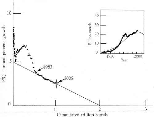
Equation B.4 then says that if you were to plot q_t/Q_t versus Q_t, the intercept on the y axis would be the parameter b and the intercept on the x axis would be the ultimate recoverable oil, Q_max. In other words, the production rate is divided by the cumulative production at any time (t) and plotted versus the cumulative production. From this plot, the intercept on the x axis is the ultimate recoverable oil. This plot can be done at any time, even before the peak rate is reached. The timing of the peak can be calculated by taking the derivative of Equation B.2 and setting it equal to zero. This leads to:

${\mathit{t}}_{\mathrm{peak}}=\frac{1}{\mathit{b}}\mathrm{l}\mathrm{n}(\mathit{a})$

To use Equation B.5, you need to know the parameter a, which was not determined from the plot of Equation B.4. The easiest way to determine the parameter a is to rearrange Equation B.1 into this form:

$\frac{{\mathit{Q}}_{\text{max}}}{{\mathit{Q}}_{\mathit{t}}}-1=\mathit{a}{\mathit{e}}^{-\mathit{bt}}$

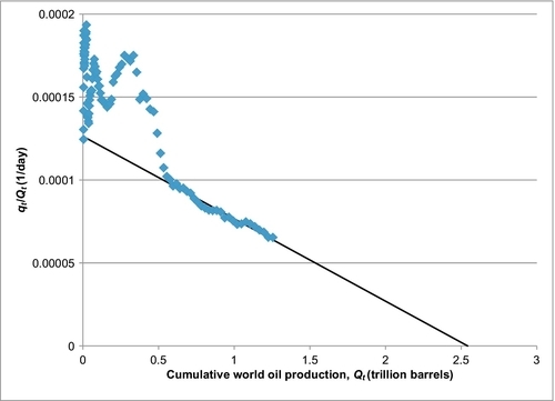
Equation B.6 says that if you plot Q_max/Q_t − 1 versus e^− bt, the slope of the plot will be equal to a. To do this second plot, I assume that I have already determined b and Q_max from the plot of Equation B.4. Deffeyes showed his plot of Equation B.4 using the world production data up until 2005, which is reproduced here as Figure B.1. His extrapolation to the x axis shows an intercept of 2 trillion barrels, which is his estimate of the ultimate recoverable oil (Q_max). Prior to 1983, the data was increasing and decreasing and had not settled down to form a straight line. From 1983 to 2005, the data dots lie on the straight line that Hubbert’s theory predicts. Deffeyes was also able to deduce his estimate for the time of the peak oil rate directly from his plot. If the ultimate recovery is projected to be 2 trillion barrels, the peak oil rate will occur when the cumulative production is 1 trillion barrels. This occurred in 2005 and led Deffeyes to predict that oil production would peak in that year.

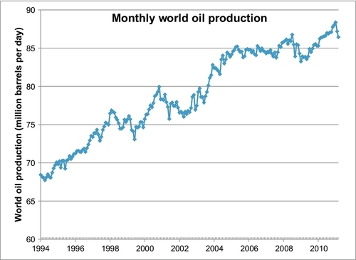
World oil production, however, did not peak in 2000 or in 2005. Figure B.2 shows annual world oil production from 1965 to 2010, and at that time, the production was still increasing. Figure B.3 shows world oil production on a monthly basis from the beginning of 1994 to early 2011, and though there are occasional declines, the overall trend on both plots is upwards and there is no evidence that a peak has occurred or will occur. The occasional dips in production that have occurred in the past 45 years are due to decreases in demand rather than decreases in supply. This does not, however, stop the pundits from declaring that world oil production has peaked every time the production decreases from one year to the next or even from one month to the next. It should be noted that Figures B.2 and B.3 use data from two different sources. The data for Figure B.2 comes from the BP Annual Statistical Review, while the data for Figure B.3 comes from the U.S. Energy Information Agency (EIA). Any discrepancies that are perceived between the two plots are due to the different data sources. What is important is that both plots show a consistent upward trend in world oil production.

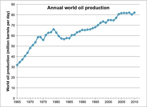
Production did show a secondary peak in 1979, and from 1979 to 1983, production did decrease. This was due to a steep increase in the world oil price in the 1970s, which resulted in decreased demand in the early 1980s as people reduced their use of transportation fuels. From 1983 to the present day, there has been a steady increase in oil demand, which has been matched by supply. The world economic crisis that was precipitated in the middle of 2008 tempered demand, which caused a decrease in production in late 2008. From January 2009 to January 2011, there was a persistent increase in production. The uprising in Libya and other countries in the Middle East in early 2011, which is being called the “2011 Arab Spring,” has once again caused a new round of price increases and a resulting decrease in demand for oil; however, this too is expected to be temporary.

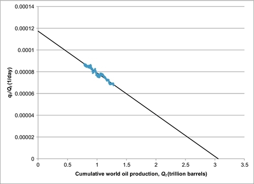
If the production data shown in Figure B.2 is plotted according to Equation B.4, the result is Figure B.4. Extrapolating this to the x-axis gives a value for Q_max of 2.54 trillion barrels, compared with the value of 2 trillion barrels that Deffeyes derived using this same data up until 2005. If the monthly data published by the EIA and shown plotted in Figure B.3 is used to do the same plot, an even more startling revelation emerges. This plot is shown in Figure B.5. This is the monthly data from January 1994 to March 2011 and comes from a very reliable source—the US Energy Information Administration. When this data is extrapolated to the x-axis, the Q_max is 3.055 trillion barrels. Of this 3 trillion barrels, 1.3 trillion barrels has already been produced. This leaves about 1.7 trillion barrels still to be found and produced. According to the EIA, the current amount of the listed world oil proved reserves is 1.3 trillion barrels, meaning that there are only 400 billion barrels still to be found. Remember, these numbers are a function of oil price and are likely to be conservative. Given that this data is probably the most reliable available data, this estimate is probably the most reliable estimate using current economics. It would seem that more oil is appearing all the time and this is due to economics. If and when the price of oil goes up again, and stays up, these numbers will increase again as well.

The value for the exponential coefficient parameter (a) is obtained using a plot of Equation B.6. Using this plot and the monthly data from EIA, a value is obtained for a:

$\mathit{a}=162.66$

This is a dimensionless parameter. The intercept on the y-axis in Figure B.5 gives a value for b:

$\mathit{b}=0.00011733{\mathrm{days}}^{-1}$

Using the above values for a and b, these numbers can be inserted into Equation B.5 to calculate an updated date for the timing of the world peak oil rate.

${\mathit{t}}_{\mathrm{peak}}=\frac{1}{\mathit{b}}ln\left(\mathit{a}\right)=\frac{1}{0.00011733}ln\left(162.66\right)=43,396\mathrm{d}\mathrm{a}\mathrm{y}\mathrm{s}$

The 43,396 days is measured from an arbitrary time zero, used in the plots of 1/1/1900. This equation gives a peak oil date of October 23, 2018. Note that I am not saying that the world oil production will peak in October 2018. I am saying that, using the Hubbert model and the latest and most accurate monthly world oil production data, the current projection for the peak oil rate is October 23, 2018. If the price of oil remained constant for the next 7 years and there were no big technological breakthroughs during that time, this may prove to be an approximately accurate forecast. I don’t expect that this will be the case and so this date will probably move again.

Hubbert’s Model for World Coal Production

Hubbert’s model can be applied to finite resources, such as coal. According to Hubbert’s model, the total cumulative production that can be expected for coal is given by the same Equation B.1:

${\mathit{Q}}_{\mathit{t}}=\frac{{\mathit{Q}}_{\text{max}}}{1+\mathit{a}{\mathit{e}}^{-\mathit{bt}}}$

Where now

Q_t = cumulative coal production at time (t) in tons

q_t = coal production rate at time (t) usually in tons/year

Q_max = ultimate cumulative coal production, in tons

a = growth or decline coefficient, dimensionless

b = growth or decline exponent, dimensions are the reciprocal of time such as 1 per year

The production rate (q_t) at any time (t) is the derivative of the cumulative and so is given by

${\mathit{q}}_{\mathit{t}}=\frac{{\mathit{Q}}_{\text{max}}\mathit{ab}{\mathit{e}}^{-\mathit{bt}}}{{\left(1+\mathit{a}{\mathit{e}}^{-\mathit{bt}}\right)}^2}$

If this model is the correct model for the production data, as long as there is early time data, the data can be fitted to the model to determine the ultimate recovery (Q_max) as well as the parameters a and b. There are several ways to determine the parameters from the data. The first method, which Hubbert recommended, was to rearrange Equations B.1 and B.2 to give:

$\frac{{\mathit{q}}_{\mathit{t}}}{{\mathit{Q}}_{\mathit{t}}}=\mathit{b}-\frac{\mathit{b}{\mathit{Q}}_{\mathit{t}}}{{\mathit{Q}}_{\text{max}}}$

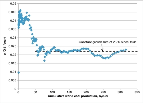
Using Equation B.3, q_t/Q_t versus Q_t is plotted. Then, the intercept on the y axis is the parameter b and the intercept on the x axis is the ultimate recoverable coal, Q_max, the ultimate cumulative coal production. The parameter, q_t/Q_t, represents the growth rate of the cumulative world coal production. This is plotted in Figure B.6, and what it shows is that the growth rate of the cumulative has been constant at about 2.2% since 1931. Moreover, it has not established a trend that can be extrapolated to an ultimate cumulative production, Q_max. The fact that this Hubbert trend has not been established suggests that perhaps the coal production peak is still many years away. Despite the failure of this method of parameter estimation, it is still possible to fit Rutledge’s data to Hubbert’s model to determine the Hubbert parameters and make a forecast of future production.

Another method of doing this is to use nonlinear regression techniques. This is not a simple task, but can be accomplished using the “Solver” function in an Excel spreadsheet.

Using the nonlinear regression method, Rutledge’s data has been fitted to Hubbert’s model, and what is obtained is the forecast shown in Figure 13.3. The red line in this chart is a plot of the Hubbert model, and the blue points are the Rutledge data points. The parameters obtained from nonlinear regression and used to plot Hubbert’s model are:

Q_max = 3529 Gt, a = 1042.15, and b = 0.02203 per year.

The timing for the peak coal production can be calculated using Equation B.5

${\mathit{t}}_{\mathrm{peak}}=\frac{1}{\mathit{b}}ln\left(\mathit{a}\right)=\frac{1}{0.02203}ln\left(1042.15\right)=315.43\mathit{y}\mathit{e}\mathit{a}\mathit{r}\mathit{s}$

Measured from 1800, this puts the peak of coal production in the year 2115. This estimate has an accuracy limited by the model fit of the data, which is about 15%. Basically, the peak could occur anywhere from 2070 to 2160.