
22 ASC 330 INVENTORY
Example of a consignment arrangement
Product financing arrangements
Sales made with the buyer having the right of return
Initial Measurement - Valuation of Inventories
Raw materials and merchandise inventory
Example of recording raw material costs
Example of allocating fixed overhead to units produced
Example of variable and fixed overhead allocation
Example of the basic principles involved in the application of FIFO
Example of the single goods (unit) LIFO approach
Example of the dollar-value LIFO method
Weighted-average and moving-average
Example of the weighted-average method
Comparison of cost flow assumptions
Example of the lower of cost or market calculation
Example of the cost-to-retail method
Example of the lower of cost or market rule – FIFO and average-cost methods
Example of the LIFO retail method
Other inventory valuation methods
Differences between GAAP and Income Tax Accounting for Inventories
Full absorption costing—income tax
Uniform capitalization rules—income tax versus GAAP
Inventory capitalization for retailers/wholesales—income tax versus GAAP
Inventories valued at selling price
Stripping costs incurred during production in the mining industry
PERSPECTIVE AND ISSUES
Subtopic
ASC 330, Inventory, consists of one subtopic:
- ASC 330-10, Overall, that provides guidance on the accounting and reporting practices on inventory.
ASC 330, Inventory, discusses the definition, valuation, and classification of inventory, as well as the measurement and classification of inventories during interim periods.
Scope
ASC 330 applies to all entities but is not necessarily applicable to:
- Not-for-profit entities
- Regulated utilities.
(ASC 330-10-15-2 and 15-3)
Overview
The accounting for inventories is a major consideration for many entities because of its significance to both the income statement (cost of goods sold) and the statement of financial position (current assets).
The complexity of accounting for inventories arises from factors that include:
- The high volume of activity (or turnover) and the associated challenges of keeping accurate, up-to-date records.
- Choosing from among various cost flow alternatives that are permitted by GAAP.
- Ensuring compliance with complex US income tax laws and regulations when electing to use the last-in, first-out (LIFO) method.
- Monitoring and properly accounting for adjustments necessitated by applying the lower of cost or market method to the inventory.
There are two types of entities for which the accounting for inventories is relevant. The merchandising entity purchases inventory for resale to its customers. The manufacturer buys raw materials, and processes those raw materials using labor and equipment into finished goods that are then sold to its customers. While the production process is progressing, the costs of the raw materials, salaries and wages paid to the labor force (and related benefits), depreciation of the machinery, and an allocated portion of the manufacturer's overhead are accumulated by the accounting system as work in process (WIP). Finished goods inventory is the completed product which is on hand awaiting shipment or sale.
In the case of either type of entity, we are concerned with answering the same basic questions.
- At what point in time should the items be included in inventory (ownership)?
- What costs incurred should be included in the valuation of inventories?
- What cost flow assumption should be used?
- At what value should inventories be reported (determination of the lower of cost or market, or LCM)?
DEFINITIONS OF TERMS
Source: ASC 330-10-20
Direct Effects of a Change in Accounting Principle. Those recognized changes in assets or liabilities necessary to effect a change in accounting principle. An example of a direct effect is an adjustment to an inventory balance to effect a change in inventory valuation method. Related changes, such as an effect on deferred income tax assets or liabilities or an impairment adjustment resulting from applying the lower-of-cost-or-market test to the adjusted inventory balance, also are examples of direct effects of a change in accounting principle.
Inventory. The aggregate of those items of tangible personal property that have any of the following characteristics:
- Held for sale in the ordinary course of business
- In process of production for such sale
- To be currently consumed in the production of goods or services to be available for sale.
The term inventory embraces goods awaiting sale (the merchandise of a trading concern and the finished goods of a manufacturer), goods in the course of production (work in process), and goods to be consumed directly or indirectly in production (raw materials and supplies). This definition of inventories excludes long-term assets subject to depreciation accounting, or goods which, when put into use, will be so classified. The fact that a depreciable asset is retired from regular use and held for sale does not indicate that the item should be classified as part of the inventory. Raw materials and supplies purchased for production may be used or consumed for the construction of long-term assets or other purposes not related to production, but the fact that inventory items representing a small portion of the total may not be absorbed ultimately in the production process does not require separate classification. By trade practice, operating materials and supplies of certain types of entities such as oil producers are usually treated as inventory.
Market. As used in the phrase lower of cost or market, the term market means current replacement cost (by purchase or by reproduction, as the case may be) provided that it meets both of the following conditions:
- Market shall not exceed the net realizable value
- Market shall not be less than net realizable value reduced by an allowance for an approximately normal profit margin.
Net Realizable Value. Estimated selling price in the ordinary course of business less reasonably predictable costs of completion and disposal.
CONCEPTS, RULES, AND EXAMPLES
Ownership of Goods
Generally, in order to obtain an accurate measurement of inventory quantity, it is necessary to determine when title legally passes between buyer and seller. The exception to this general rule arises from situations when the buyer assumes the significant risks of ownership of the goods prior to taking title and/or physical possession of the goods. Substance over form in this case would dictate that the inventory is an asset of the buyer and not the seller, and that a purchase and sale of the goods be recognized by the parties irrespective of the party that holds legal title.
The most common error made in this area is to assume that an entity has title only to the goods it physically holds. This may be incorrect in two ways:
- Goods held may not be owned, and
- Goods that are not held may be owned.
Four issues affect the determination of ownership:
- Goods in transit,
- Consignment arrangements,
- Product financing arrangements, and
- Sales made with the buyer having the right of return.
Goods in transit.
At year-end, any goods in transit from seller to buyer must be included in one of those parties' inventories based on the conditions of the sale. Such goods are included in the inventory of the firm financially responsible for transportation costs. This responsibility may be indicated by a variety of peculiar shipping acronyms such as FOB, which is used in overland shipping contracts, or FAS, CIF, C&F, and ex-ship, which are used in maritime contracts.
The term FOB is an abbreviation of “free on board.” If goods are shipped FOB destination, transportation costs are paid by the seller and title does not pass until the carrier delivers the goods to the buyer. These goods are part of the seller's inventory while in transit. If goods are shipped FOB shipping point, transportation costs are paid by the buyer and title passes when the carrier takes possession of the goods. These goods are part of the buyer's inventory while in transit. The terms FOB destination and FOB shipping point often indicate a specific location at which title to the goods is transferred, such as FOB Cleveland. This means that the seller retains title and risk of loss until the goods are delivered to a common carrier in Cleveland who will act as an agent for the buyer. The rationale for these determinations originates in agency law, since transfer of title is conditioned upon whether the carrier with physical possession of the goods is acting as an agent of the seller or the buyer.
A seller who ships FAS (free alongside) must bear all expense and risk involved in delivering the goods to the dock next to (alongside) the vessel on which they are to be shipped. The buyer bears the costs of loading and shipment. Title passes when the carrier, as agent for the buyer, takes possession of the goods.
In a CIF (cost, insurance, and freight) contract, the buyer agrees to pay in a lump sum the cost of the goods, insurance costs, and freight charges. In a C&F (cost and freight) contract, the buyer promises to pay a lump sum that includes the cost of the goods and all freight charges. In either case, the seller must deliver the goods to the buyer's agent/carrier and pay the costs of loading. Both title and risk of loss pass to the buyer upon delivery of the goods to the carrier.
A seller who delivers goods ex-ship bears all expense and risk until the goods are unloaded, at which time both title and risk of loss pass to the buyer.
The Meridian Vacuum Company is located in Santa Fe, New Mexico, and obtains compressors from a supplier in Hong Kong. The standard delivery terms are free alongside (FAS) a container ship in Hong Kong harbor, so that Meridian takes legal title to the delivery once possession of the goods is taken by the carrier's dockside employees for the purpose of loading the goods on board the ship. When the supplier delivers goods with an invoiced value of $120,000 to the wharf, it e-mails an advance shipping notice (ASN) and invoice to Meridian via an electronic data interchange (EDI) transaction, itemizing the contents of the delivery. Meridian's computer system receives the EDI transmission, notes the FAS terms in the supplier file, and therefore automatically logs it into the company computer system with the following entry:
![]()
The goods are assigned an “In Transit” location code in Meridian's perpetual inventory system. When the compressor eventually arrives at Meridian's receiving dock, the receiving staff records a change in inventory location code from “In Transit” to a code designating a physical location within the warehouse.
Meridian's secondary compressor supplier is located in Vancouver, British Columbia, and ships overland using free on board (FOB) Santa Fe terms, so the supplier retains title until the shipment arrives at Meridian's location. This supplier also issues an advance shipping notice by EDI to inform Meridian of the estimated arrival date, but in this case Meridian's computer system notes the FOB Santa Fe terms, and makes no entry to record the transaction until the goods arrive at Meridian's receiving dock.
Consignment arrangements.
In consignment arrangements, the consignor ships goods to the consignee, who acts as the agent of the consignor in trying to sell the goods. In some consignments, the consignee receives a commission upon sale of the goods to its customer. In other arrangements, the consignee “purchases” the goods simultaneously with the sale of the goods to the customer. Goods on consignment are included in the inventory of the consignor and excluded from the inventory of the consignee.
The Portable Handset Company (PHC) ships a consignment of its cordless phones to a retail outlet of the Consignee Corporation. PHC's cost of the consigned goods is $3,700. PHC shifts the inventory cost into a separate inventory account to track the physical location of the goods. The entry follows:
![]()
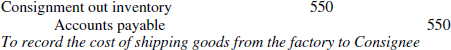
A third-party shipping company ships the cordless phone inventory from PHC to Consignee. Upon receipt of an invoice for this $550 shipping expense, PHC charges the cost to consignment inventory with the following entry:
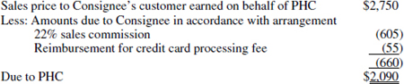
Consignee sells half the consigned inventory during the month for $2,750 in credit card payments, and earns a 22% commission on these sales, totaling $605. According to the consignment arrangement, PHC must also reimburse Consignee for the 2% credit card processing fee, which is $55 ($2,750 × 2%). The results of this sale are summarized as follows:
Upon receipt of the monthly sales report from Consignee, PHC records the following entries:
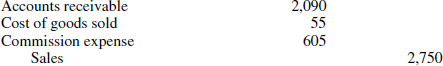
To record the sale made by Consignee acting as agent of PHC, the commission earned by Consignee and the credit card fee reimbursement earned by Consignee in connection with the sale
![]()
To transfer the related inventory cost to cost of goods sold, including half the original inventory cost and half the cost of the shipment to consignee [($3,700 + $550 = $4,250) × ½ = $2,125]
Product financing arrangements.
ASC 470-40 addresses the issues involved with product financing arrangements. A product financing arrangement is a transaction in which an entity (referred to as the “sponsor”) simultaneously sells and agrees to repurchase inventory to and from a financing entity. The repurchase price is contractually fixed at an amount equal to the original sales price plus the financing entity's carrying and financing costs. The purpose of the transaction is to enable the sponsor enterprise to arrange financing of its original purchase of the inventory.
FASB ruled that the substance of this transaction is that of a borrowing transaction, not a sale. That is, the transaction is, in substance, no different from the sponsor directly obtaining third-party financing to purchase inventory. ASC 470-40 specifies that the proper accounting by the sponsor is to record a liability in the amount of the selling price when the funds are received from the financing entity in exchange for the initial transfer of the inventory. The sponsor proceeds to accrue carrying and financing costs in accordance with its normal accounting policies. These accruals are eliminated and the liability satisfied when the sponsor repurchases the inventory. The inventory is not removed from the statement of financial position of the sponsor and a sale is not recorded. Thus, although legal title has passed to the financing entity, for purposes of measuring and valuing inventory, the inventory is considered to be owned by the sponsor.
For more information, see the chapter on ASC 470.
Sales made with the buyer having the right of return.
Another issue requiring special consideration exists when a buyer is granted a right of return, as defined by ASC 605-15. The seller must consider the propriety of recognizing revenue at the point of sale under such a situation. The sale is recorded only when six specified conditions are met including the condition that the future amount of returns can be reasonably estimated by the seller. If a reasonable estimate cannot be made, then the sale is not recorded until the earlier of the expiration date of the return privilege or the date when all six conditions are met. Similar to product financing costs, this situation results in the seller continuing to include the goods in its measurement and valuation of inventory even though legal title has passed to the buyer. For more information see chapter on ASC 605.
Accounting for Inventories
A major objective of accounting for inventories is the matching of appropriate costs to the period in which the related revenues are earned in order to properly compute gross profit, also referred to as gross margin. Inventories are recorded in the accounting records using either a periodic or perpetual system.
In a periodic inventory system, inventory quantities are determined by physical count. The quantity of each item counted is then priced using the cost flow assumption that the enterprise had adopted as its accounting policy for that type of inventory. Cost of goods sold is computed by adding beginning inventory and net purchases (or cost of goods manufactured) and subtracting ending inventory.
A perpetual inventory system keeps a running total of the quantity (and possibly the cost) of inventory on hand by maintaining subsidiary inventory records that reflect all sales and purchases as they occur. When inventory is purchased, inventory (rather than purchases) is debited. When inventory is sold, the cost of goods sold and corresponding reduction of inventory are recorded.
Using a periodic inventory system necessitates the taking of physical inventory counts to determine the quantity of inventory on hand at the end of a reporting period. To facilitate accurate annual financial statements, in practice physical counts are performed at least annually on the last day of the fiscal year.
If the enterprise maintains a perpetual inventory system, it must regularly and systematically verify the accuracy of its perpetual records by physically counting inventories and comparing the quantities on hand with the perpetual records. GAAp does not provide explicit requirements regarding the timing and frequency of physical counts necessary to verify the perpetual records; however there is a US income tax requirement (IRC§47l[b][1]) that a taxpayer perform “... a physical count of inventories at each location on a regular and consistent basis....” The purpose of this requirement is to enable the taxpayer to support any tax deductions taken for inventory shrinkage if it elects not to take a complete physical inventory at all locations on the last day of the fiscal year. The IRS, in its Rev. Proc. 98-29, provided a “retail safe harbor method” that permits retailers to deduct estimated shrinkage where the retailer takes physical inventories at each location at least annually. (ASC 330-10-30-1)
Initial Measurement - Valuation of Inventories
The primary basis of accounting for inventories is cost. Cost is defined as the sum of the applicable expenditures and charges directly or indirectly incurred in bringing an article to its existing condition and location. This definition allows for a wide interpretation of the costs to be included in inventory.
Raw materials and merchandise inventory.
For raw materials and merchandise inventory which are purchased outright, the identification of cost is relatively straightforward. The cost of these purchased inventories will include all expenditures incurred in bringing the goods to the point of sale and converting them to a salable condition. These costs include the purchase price, transportation costs (freight-in), insurance while in transit, and handling costs charged by the supplier.
Aruba Bungee Cords, Inc. (ABC) purchases rubber bands, a raw material that it uses in manufacturing its signature product. The company typically receives delivery of all its raw materials and uses them in manufacturing its finished products during the winter, and then sells its stock of finished goods in the spring. The supplier invoice for a January delivery of rubber bands includes the following line items:
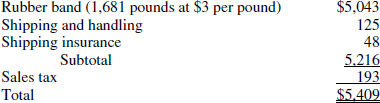
Since ABC is using the rubber bands as raw materials in a product that it resells, it will not pay the sales tax. However, both the shipping and handling charge and the shipping insurance are required for ongoing product acquisition, and so are included in the following entry to record receipt of the goods:
![]()
On February 1, ABC purchases a $5,000, two-month shipping insurance policy (paradoxically, this type of policy is sometimes referred to as “inland marine” coverage) that applies to all incoming supplier deliveries for the remainder of the winter production season, allowing it to refuse shipping insurance charges on individual deliveries. Since the policy insures all inbound raw materials deliveries (not just rubber bands), it is too time-consuming to charge the cost of this policy to individual raw material deliveries using specific identification, and accordingly, the controller can estimate a flat charge per delivery based on the number of expected deliveries during the two-month term of the insurance policy as follows:
$5,000 insurance premium ÷ 200 expected deliveries during the policy term = $25 per delivery and then charge each delivery with $25 as follows:
![]()
To allocate cost of inland marine coverage to inbound insured raw materials shipments
In this case, however, the controller determined that shipments are expected to occur evenly during the two-month policy period and therefore will simply make a monthly standard journal entry as follows:
![]()
To amortize premium on inland marine policy using the straight-line method
Note that the controller must be careful, under either scenario, to ensure that perpetual inventory records appropriately track unit costs of raw materials to include the cost of shipping insurance. Failure to do so would result in an understatement of the cost of raw materials inventory on hand at the end of any accounting period.
Purchases can be recorded at their gross amount or net of any allowable discount. If recorded gross, the discounts taken represent a reduction in the purchase cost for purposes of determining cost of goods sold. On the other hand, if they are recorded net, any lost discounts are treated as a financial expense, not as cost of goods sold. The net method is considered to be theoretically preferable, but the gross method is simpler and, thus, more commonly used. Either method is acceptable under GAAP, provided that it is consistently applied.
Inventory purchases and sales with the same counterparty. Some enterprises sell inventory to another party from whom they also acquire inventory in the same line of business. These transactions may be part of a single or separate arrangements and the inventory purchased or sold may be raw materials, work-in-process, or finished goods. These arrangements require careful analysis to determine if they are to be accounted for as a single exchange transaction under ASC 845, Nonmonetary Transactions, and whether they are to be recognized at fair value or at the carrying value of the inventory transferred.1 More detailed information can be found in the chapter on ASC 845.
Inventory hedges.
One notable exception to recording inventories at cost is provided by the hedge accounting requirements of ASC 815. If inventory has been designated as the hedged item in a fair value hedge, changes in the fair value of the hedged inventory are recognized on the statement of financial position as they occur, with the offsetting charge or credit recognized currently in net income. Hedging is discussed in detail in Chapter 10.
Manufacturing inventories.
Inventory cost in a manufacturing enterprise includes both acquisition and production costs. This concept is commonly referred to as full absorption or full costing. As a result, the WIP and finished goods inventories include direct materials, direct labor, and an appropriately allocated portion of indirect production costs referred to as indirect overhead.
Under full absorption costing, indirect overhead costs—costs that are incidental to and necessary for production—are allocated to goods produced and, to the extent those goods are uncompleted or unsold at the end of a period, are included in ending WIP or finished goods inventory, respectively. Indirect overhead costs include such costs as
- Depreciation and cost depletion
- Repairs
- Maintenance
- Factory rent and utilities
- Indirect labor
- Normal rework labor, scrap, and spoilage
- Production supervisory wages
- Indirect materials and supplies
- Quality control and inspection
- Small tools not capitalized.
Indirect overhead is comprised of two elements, variable and fixed overhead. ASC 330-10-30-3 clarifies that variable overhead is to be allocated to work-in-process and finished goods based on the actual usage of the production facilities. Fixed overhead, however, is to be allocated to work-in-process and finished goods based on the normal expected capacity of the enterprise's production facilities, with the overhead rate recomputed in instances when actual production exceeds the normal capacity. Initially, this may appear to be an inconsistent accounting method; however, the use of this convention ensures that the inventory is not recorded at an amount in excess of its actual cost, as illustrated in the following example:
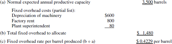
Brewed Refreshment Plant, Inc. (BRP), located in Washington, D.C., has historically produced between 3,200 and 3,800 barrels of beer annually with its average production approximating 3,500 barrels. This average takes into account its normal number of work shifts and the normal operation of its machinery adjusted for downtime for normal maintenance and recalibration. BRP's average capacity and overhead costs (partial list) are presented below.
Scenario 1: The Washington Nationals major-league baseball team outperforms expectations; since BRP's beer is sold at the Nationals' stadium, BRP substantially increases production beyond the normal level expected.
![]()
If BRP were to apply fixed overhead using the rate based on its normal productive capacity, the calculation would be as follows:
4,500 barrels produced × $0.4229 per barrel = $1,903 of overhead applied
This would result in an over-allocation of $423, the difference between the $1,903 of overhead applied and the $1,480 of overhead actually incurred. This violates the lower of cost or market principle, since the inventory would be valued at an amount that exceeded its actual cost. Therefore, BRP applied ASC 330 and recomputed its fixed overhead rate as follows:
1,480 fixed overhead incurred ÷ Revised production level of 4,500 barrels = $0.3289 per barrel
Scenario 2: The Washington Nationals experience a cold, rainy summer and worse-than-expected attendance. If production lags expectations and BRP only produces 2,500 barrels of beer, the original overhead rate is not revised. The fixed overhead is allocated as follows:
2,500 barrels produced × $0.4229 per barrel = $1,057 of overhead applied
Per ASC 330, when production levels decline below the original expectation, the fixed overhead rate is not recomputed. The $423 difference between the $1,480 of actual fixed overhead incurred and the $1,057 of overhead applied is accounted for as an expense in the period incurred.
For the purpose of determining normal productive capacity, it is expected that capacity will vary from period to period based on enterprise-specific or industry-specific experience. Management is to formulate a judgment regarding a reasonable range of normal production levels expected to be achieved under normal operating conditions.
The enterprise may incur unusually large expenses resulting from idle facilities, excessive waste, spoilage, freight, or handling costs. ASC 330 clarifies that when this situation occurs, the abnormal portion of these expenses is to be treated as a cost of the period incurred and not to be allocated to inventory.
Generally, interest costs incurred during the production of inventory are not capitalized under ASC 835-20. A complete discussion regarding the capitalization of interest costs is provided in the chapter on ASC 835.
The InCase Manufacturing Company (IMC) uses injection molding to create two types of plastic CD cases—regular size and mini—on a seven-day, three-shift production schedule. During the current month, it records the following overhead expenses:
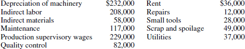
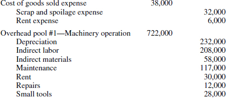
IMC's controller analyzed scrap and spoilage statistics and determined that abnormal losses of $32,000 were incurred due to a bad batch of plastic resin pellets. She adjusted scrap and spoilage expense by charging the cost of those pellets to cost of goods sold during the current period, resulting in a reduced scrap and spoilage expense of $17,000. Also, the rent cost includes a $6,000 lease termination penalty payable to the lessor of a vacant factory. Since this cost is considered an exit or disposal activity under ASC 420, it does not benefit production and is therefore charged directly to expense in the current period.
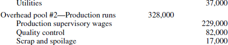
For allocation purposes, IMC's controller elects to group the adjusted overhead expenses into two cost pools. Pool #1 contains all expenses related to machinery operation, which includes depreciation, indirect labor, indirect materials, maintenance, rent, repairs, small tools, and utilities. Pool #2 contains all expenses related to production runs, which includes production supervisory wages, quality control, scrap, and spoilage. The following three journal entries record (1) the recognition of excess scrap and unused facilities in the current period, (2) the allocation of costs to the machinery cost pool, and (3) the allocation of costs to the production runs cost pool:
Since the costs in overhead pool #1 are centered on machine usage, the controller elects to use the total operating hours used for the production of each product as the allocation basis for that pool. The accumulated production hours by machine for the past month are as follows:
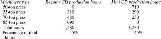
Since the costs in overhead pool #2 are centered on production volume, the controller decides to use the total pounds of plastic resin pellets used for production during the month as the allocation basis for that cost pool. The total plastic resin usage, adjusted for spoilage, was 114,000 pounds of resin for the regular CD cases and 76,000 pounds for the mini CD cases, which is a percentage split of 60% for regular CD cases and 40% for mini CD cases.
With the calculation of allocation bases completed, the split of overhead costs between the two products follows:
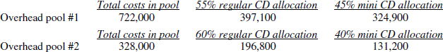
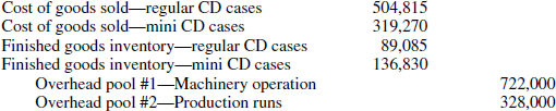
Thus, the total overhead allocated to regular CD cases is $593,900 (397,100 + 196,800), while the total overhead allocated to mini CD cases is $456,100 (324,900 + 131,200). Of the case quantities produced, 85% of the regular CD cases and 70% of the mini CD cases were sold during the month, with the remainder being transferred into finished goods inventory. IMC's controller uses these percentages to apportion the cost of allocated overhead between the cost of goods sold and finished goods inventory, as shown in the following entry:
Determining inventory cost.
The theoretical basis for valuing inventories and cost of goods sold requires assigning production and/or acquisition costs to the specific goods to which they relate. This method of inventory valuation is usually referred to as specific identification. Specific identification is generally not practical inasmuch as the product will generally lose its separate identity as it passes through the production and sales process. Exceptions to this would arise in situations involving small inventory quantities with high unit value and low turnover rate, such as automobiles or heavy machinery. Because of the limited applicability of specific identification, it is necessary to make certain assumptions regarding the cost flows associated with inventory. Although these cost flow assumptions are used for accounting purposes, they may or may not reflect the actual physical flow of the inventory.
Cost flow assumptions.
The most common cost flow assumptions used are specified in ASC 330-10-30-9:
- first-in, first-out (FIFO),
- last-in, first-out (LIFO), and
- weighted-average.
Additionally, there are variations in the application of each of these assumptions which are commonly used in practice. ASC 330-10-30-9 points out that:
“The major objective in selecting a method should be to choose the one which, under the circumstances, most clearly reflects periodic income.”
In selecting which cost flow assumption to adopt as its accounting policy for a particular type of industry, management should consider a variety of factors. First, the industry norm should be examined, as this will facilitate intercompany comparison by financial statement users. The appropriateness of using a particular cost flow assumption will vary depending on the nature of the industry and the expected economic climate. The appropriate method in a period of rising prices differs from the method that is appropriate for a period of declining prices. Each of the foregoing assumptions and their relative advantages or disadvantages are discussed below. Examples are provided to enhance understanding of the application.
First-in, first-out (FIFO).
The FIFO method of inventory valuation assumes that the first goods purchased are the first goods used or sold, regardless of the actual physical flow. This method is thought to most closely parallel the physical flow of the units in most industries. The strength of this cost flow assumption lies in the inventory amount reported on the statement of financial position. Because the earliest goods purchased are the first ones removed from the inventory account, the remaining balance is composed of items priced at more recent cost. This yields results similar to those obtained under current cost accounting on the statement of financial position. However, the FIFO method does not necessarily reflect the most accurate income figure as older, historical costs are being charged to cost of goods sold and matched against current revenues.
Given this data, the cost of goods sold and ending inventory balance are determined as follows:
Notice that the total of the units in cost of goods sold and ending inventory, as well as the sum of their total costs, is equal to the goods available for sale and their respective total costs.
The FIFO method provides the same results under either the periodic or perpetual inventory tracking system.
Last-in, first-out (LIFO).
The LIFO method of inventory valuation assumes that the last goods purchased are the first goods used or sold. This allows the matching of current costs with current revenues and provides the best measure of gross profit. However, unless costs remain relatively unchanged over time, the LIFO method will usually misstate the ending inventory statement of financial position amount, because LIFO inventory usually includes costs of acquiring or manufacturing inventory that were incurred in earlier periods. LIFO does not usually follow the physical flow of merchandise or materials. However, the matching of physical flow with cost flow is not an objective of accounting for inventories.
LIFO accounting is actually an income tax concept. Consequently, the rules regarding the application of the LIFO method are not set forth in US GAAP, but rather, are found in the US Internal Revenue Code (IRC) §472. US Treasury regulations provide that any taxpayer that maintains inventories may select LIFO application for any or all inventoriable items. This election is made with the taxpayer's income tax return on Form 970 after the close of the first tax year that the taxpayer intends to use (or expand the use of) the LIFO method.
The quantity of ending inventory on hand at the beginning of the year of election is termed the “base layer.” This inventory is valued at actual (full absorption) cost, and unit cost for each inventory item is determined by dividing total cost by the quantity on hand. At the end of the initial and subsequent years, increases in the quantity of inventory on hand are referred to as increments, or LIFO layers. These increments are valued individually by applying one of the following costing methods to the quantity of inventory representing a layer:
- The actual cost of the goods most recently purchased or produced
- The actual cost of the goods purchased or produced in order of acquisition
- An average unit cost of all goods purchased or produced during the current year
- A hybrid method that more clearly reflects income (for income tax purposes, this method must meet with the approval of the IRS Commissioner).
Thus, after using the LIFO method for five years, it is possible that an enterprise could have ending inventory consisting of the base layer and five additional layers (or increments) provided that the quantity of ending inventory increased every year.
Rose Co. is in its first year of operation and elects to use the periodic LIFO method of inventory valuation. The company sells only one product. Rose applies the LIFO method using the order of current year acquisition cost. The following data are given for years 1 through 3:
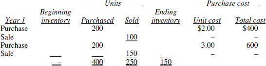
In year 1 the following occurred:
- The total goods available for sale were 400 units.
- The total sales were 250 units.
- Therefore, the ending inventory was 150 units.
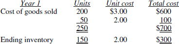
The ending inventory is valued at the earliest current year acquisition cost of $2.00 per unit. Thus, ending inventory is valued at $300 (150 × $2.00).
Another way to look at this is to analyze both cost of goods sold and ending inventory.
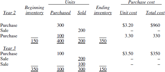
Note that the base-year cost is $2.00 and that the base-year level is 150 units. Therefore, if ending inventory in the subsequent period exceeds 150 units, a new layer (or increment) will be created.
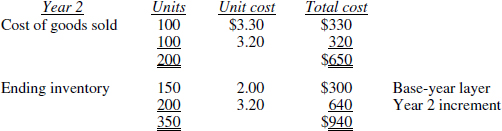
If ending inventory exceeds 350 units in the next period, a third layer (increment) will be created.
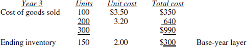
Notice how the decrease (decrement) of 200 units in year 3 eliminated the entire year 2 increment. Thus, any year 4 increase in the quantity of inventory would result in a new increment, which would be valued at year 4 prices.
In situations where the ending inventory decreases from the level established at the close of the preceding year, the enterprise experiences a decrement or LIFO liquidation. Decrements reduce or eliminate previously established LIFO layers. Once any part of a LIFO layer has been eliminated, it cannot be reinstated after year-end. For example, if in its first year after the election of LIFO an enterprise establishes a LIFO layer (increment) of ten units, then in the next year inventory decreases by four units, leaving the first layer at six units, the enterprise is not permitted in any succeeding year to increase the number of units in the first year layer back up to the original ten units. The quantity in the first layer remains at a maximum of six units subject to further reduction if decrements occur in future years. Any unit increases in future years will create one or more new layers. The effect of LIFO liquidations in periods of rising prices is to transfer, from ending inventory into cost of goods sold, costs that are below the current cost being paid. Thus, the resultant effect of a LIFO liquidation is to increase income for both accounting and income tax purposes. Because of this, LIFO is most commonly used by companies in industries in which levels of inventories are consistently maintained or increased over time.
LIFO liquidations can be either voluntary or involuntary. A voluntary liquidation occurs when an enterprise deliberately lets its inventory levels drop. Voluntary liquidations may be desirable for a number of reasons. Management might consider the current price of purchasing the goods to be too high, a smaller quantity of inventory might be needed for efficient production due to conversion to a “just-in-time” production model, or inventory items may have become obsolete due to new technology or transitions in the enterprise's product lines.
Involuntary LIFO liquidations stem from reasons beyond the control of management, such as a strike, material shortages, shipping delays, etc. Whether voluntary or involuntary, all LIFO liquidations result in a corresponding increase in income in periods of rising prices.
To determine the effect of the liquidation, management must compute the difference between actual cost of sales and what cost of sales would have been had the inventory been reinstated. The Internal Revenue Service has ruled that this hypothetical reinstatement must be computed under the company's normal pricing procedures for valuing its LIFO increments. In the preceding example the effect of the year 3 LIFO liquidation would be computed as follows:
Hypothetical inventory reinstatement
200 units @ $3.50 − $3.20 = $60
Hypothetically, if there had been an increment instead of a decrement in year 3 and the year 2 inventory layer had remained intact, 200 more units (out of the 300 total units sold in year 3) would have been charged to cost of goods sold at the year 3 price of $3.50 instead of the year 2 price of $3.20. Therefore, the difference between $3.50 and the actual amount charged to cost of sales for these 200 units liquidated ($3.20) measures the effect of the liquidation.
The following is considered acceptable GAAP disclosure in the event of a LIFO liquidation:
During 2013, inventory quantities were reduced below their levels at December 31, 2012. As a result of this reduction, LIFO inventory costs computed based on lower prior years' acquisition costs were charged to cost of goods sold. If this LIFO liquidation had not occurred and cost of sales had been computed based on the cost of 2013 purchases, cost of goods sold would have increased by approximately $xxx and net income decreased by approximately $xx or $x per share.
Applying the unit LIFO method requires a substantial amount of recordkeeping. The recordkeeping becomes more burdensome as the number of products increases. For this reason a “pooling” approach is often used to compute LIFO inventories.
Pooling is the process of grouping items that are naturally related and then treating this group as a single unit in determining LIFO cost. Because the ending inventory normally includes many items, decreases in one item can be offset by increases in others, whereas under the unit LIFO approach a decrease in any one item results in a liquidation of all or a portion of a LIFO layer.
Complexity in applying the pooling method arises from the income tax regulations. These regulations require that the opening and closing inventories of each type of good be compared. In order to be considered comparable for this purpose, inventory items must be similar as to character, quality, and price. This qualification has generally been interpreted to mean identical. The effect of this interpretation is to require a separate pool for each item under the unit LIFO method. To provide a simpler, more practical approach to applying LIFO and allow for increased use of LIFO pools, election of the dollar-value LIFO method is permitted.
Dollar-value LIFO. Dollar-value LIFO may be elected by any taxpayer. Under the dollar-value LIFO method of inventory valuation, the cost of inventories is computed by expressing base-year costs in terms of total dollars rather than specific prices of specific units. The dollar-value method also provides an expanded interpretation of the use of LIFO pools. Increments and decrements are treated the same as under the unit LIFO approach but are reflected only in terms of a net increment or liquidation for the entire pool.
Identifying pools. Three alternatives exist for determining pools under dollar-value LIFO: (1) the natural business unit method, (2) the multiple pooling method, and (3) pools for wholesalers, retailers, jobbers, and the like.
The natural business unit is defined by the existence of separate and distinct processing facilities and operations and the maintenance of separate income (loss) records. The concept of the natural business unit is generally dependent upon the type of product being produced, not the various stages of production for that product. Thus, the pool of a manufacturer can (and will) contain raw materials, WIP, and finished goods. The three examples below, adapted from the treasury regulations, illustrate the application of the natural business unit concept.
A corporation manufactures, in one division, automatic clothes washers and dryers of both commercial and domestic grade as well as electric ranges and dishwashers. The corporation manufactures, in another division, radios and television sets. The manufacturing facilities and processes used in manufacturing the radios and television sets are distinct from those used in manufacturing the automatic clothes washers, etc. Under these circumstances, an enterprise consisting of two business units and two pools would be appropriate: one consisting of all of the LIFO inventories involved with the manufacture of clothes washers and dryers, electric ranges and dishwashers and the other consisting of all the LIFO inventories involved with the production of radios and television sets.
A taxpayer produces plastics in one of its plants. Substantial amounts of the production are sold as plastics. The remainder of the production is shipped to a second plant of the taxpayer for the production of plastic toys which are sold to customers. The taxpayer operates its plastics plant and toy plant as separate divisions. Because of the different product lines and the separate divisions, the taxpayer has two natural business units.
A taxpayer is engaged in the manufacture of paper. At one stage of processing, uncoated paper is produced. Substantial amounts of uncoated paper are sold at this stage of processing. The remainder of the uncoated paper is transferred to the taxpayer's finishing mill where coated paper is produced and sold. This taxpayer has only one natural business unit, since coated and uncoated paper are within the same product line.
The treasury regulations require that a pool consist of all items entering into the entire inventory investment of a natural business unit, unless the taxpayer elects to use the multiple-pooling method.
The multiple-pooling method is the grouping of “substantially similar” items. In determining substantially similar items, consideration is given to the processing applied, the interchangeability, the similarity of use, and the customary practice of the industry. While the election of multiple pools will necessitate additional recordkeeping, it may result in a better estimation of gross profit and periodic net income.
According to Reg. §1.472-8(c), inventory items of wholesalers, retailers, jobbers, and distributors are to be assigned to pools by major lines, types, or classes of goods. The natural business unit method may be used with permission of the Commissioner.
All three methods of pooling allow for a change in the components of inventory over time. New items which properly fall within the pool may be added, and old items may disappear from the pool, but neither will necessarily cause a change in the total dollar value of the pool.
Computing dollar-value LIFO. The purpose of the dollar-value LIFO method of valuing inventory is to convert inventory priced at end-of-year prices to that same quantity of inventory priced at base-year (or applicable LIFO layer) prices. The dollar-value method achieves this result through the use of a conversion price index. The inventory computed at current year cost is divided by the appropriate index to arrive at its base-year cost. The main computational focus is on the determination of the conversion price index. There are four types of methods that can be used in the computation of the ending inventory amount of a dollar-value LIFO pool: (1) double-extension, (2) link-chain, (3) indexing, and (4) alternative LIFO for automobile dealers.
Double-extension method. This method was originally developed to compute the conversion price index. It involves extending the entire quantity of ending inventory for the current year at both base-year prices and end-of-year prices to arrive at a total dollar value for each, hence the title “double-extension.” The dollar total computed at end-of-year prices is then divided by the dollar total computed at base-year prices to arrive at the index, usually referred to as the conversion price index. This index indicates the relationship between the base-year and current prices in terms of a percentage. Each layer (or increment) is valued at its own percentage. Although a representative sample is allowed (meaning that not all of the items need to be double-extended; this is discussed in more detail under indexing), the recordkeeping under this method is very burdensome. The base-year price must be maintained for each inventory item. Depending upon the number of different items included in the inventory of the enterprise, the necessary records may be too detailed to keep past the first year or two.
The following example illustrates the double-extension method of computing the LIFO value of inventory. The example presented is relatively simple and does not attempt to incorporate all of the complexities of LIFO inventory accounting.
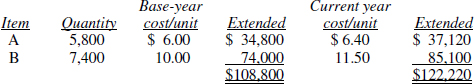
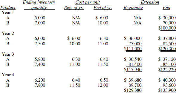
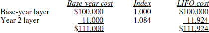
Isaacson, Inc. uses the dollar-value method of LIFO inventory valuation and computes its price index using the double-extension method. Isaacson has a single pool that contains two inventory items, A and B. Year 1 is the company's initial year of operations. The following information is given for years 1 through 4:
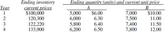
In year 1 there is no computation of an index; the index is 100%. The LIFO cost is the same as the actual current year cost. This is the base year.
In year 2 the first step is to double-extend the quantity of ending inventory at base-year and current year costs.
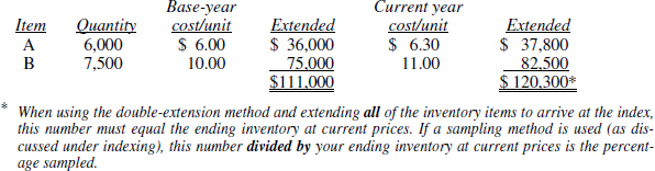
Now we can compute the conversion price index which is
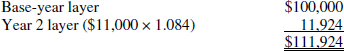
Next, compute the year 2 layer at base-year cost by taking the current year-ending inventory at base-year prices (if you only extend a sample of the inventory, this number is arrived at by dividing the ending inventory at current year prices by the conversion price index) of $111,000 and subtracting the base-year cost of $100,000. In year 2 we have an increment (layer) of $11,000 valued at base-year costs.
The year 2 layer of $11,000 at base-year cost must be converted so that the layer is valued at the prices in effect when it came into existence (i.e., at year 2 prices). This is done by multiplying the increment at base-year cost ($11,000) by the rounded conversion price index (1.084). The result is the year 2 layer at LIFO prices.
In year 3 the same basic procedure is followed.
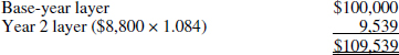
There has been a decrease in the base-year cost of the ending inventory ($111,000 − $108,800 = $2,200) which is referred to as a decrement. A decrement results in the decrease (or elimination) of previously provided layers. In this situation, the computation of the index is not necessary as there is no LIFO layer that requires a valuation. If a sampling approach has been used, the index is needed to arrive at the ending inventory at base-year cost and thus determine if there has been an increment or decrement.
Now the ending inventory at base-year cost is $108,800. The base-year cost layer is still intact at $100,000, so the cumulative increment is $8,800. Since this is less than the $11,000 increment of year 2, no additional increment is established in year 3. The LIFO cost of the inventory is shown below.
The fourth year then follows the same steps.
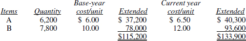
The conversion price index is 116.2% (133,900/115,200).
A current year increment exists because the ending inventory at base-year prices in year 4 of $115,200 exceeds the year 3 number of $108,800. The current year increment of $6,400 must be valued at year 4 prices. Thus, the LIFO cost of the year 4 inventory is
It is important to point out that once a layer is reduced or eliminated it is never reinstated (as with the year-2 increment) after year-end.
Link-chain method. Since the double-extension method computations are arduous even if only a few items exist in the inventory, consider the complexity that arises when there is a constant change in the inventory mix or when there is a large number of inventory items. The link-chain method of applying dollar-value LIFO was developed to mitigate the effects of this complexity.
Consider the situation where the components of inventory are constantly changing. The regulations require that any new products added to the inventory be recorded at base-year prices. If these are not available, then the earliest cost available after the base year is used. If the item was not in existence in the base year, the taxpayer may reconstruct the base cost, using a reasonable method to determine what the cost would have been if the item had been in existence in the base year. Finally, as a last resort, the current year purchase price can be used. While this does not appear to be a problem on the surface, imagine a base period that is twenty-five to fifty years in the past. The difficulty involved with finding the base-year cost may require using a more current cost, thus eliminating some of the LIFO benefit. Imagine a situation faced by a company in a “high-tech” industry where inventory is continually being replaced by newer, more advanced products. The effect of this rapid change under the double-extension method (because the new products did not exist in the base period) is to use current prices as base-year costs. When inventory has such a rapid turnover, the overall LIFO advantage becomes diluted as current and base-year costs are often identical. This situation necessitated the development of the link-chain method.
The link-chain method was originally developed for (and limited to) those companies that wanted to use LIFO but, because of a substantial change in product lines over time, were unable to reconstruct or maintain the historical records necessary to make accurate use of the double extension method. It is important to note that the double-extension and link-chain methods are not elective alternatives for the same situation. For income tax purposes, the link-chain election requires that substantial changes in product lines be evident over the years, and may not be elected solely because of its ease of application. The double-extension and index methods must be demonstrably impractical in order to elect the link-chain method. However, an enterprise may use different computational techniques for financial reporting and income tax purposes. Therefore, the link-chain method could be used for financial reporting purposes even if a different application is used for income tax purposes. Obviously, the recordkeeping burdens imposed by using different LIFO methods for GAAP and income tax purposes (including the deferred income tax accounting that would be required for the temporary difference between the GAAP and income tax bases of the LIFO inventories) would make this a highly unlikely scenario.
The link-chain method is the process of developing a single cumulative index which is applied to the ending inventory amount priced using beginning-of-the-year costs. Thus, the index computed at the end of each year is “linked” to the index from all previous years. A separate cumulative index is used for each pool regardless of the variations in the components of these pools over the years. Technological change is accommodated by the method used to calculate each current year's index. The index is calculated by double-extending a representative sample of items in the pool at both beginning-of-year prices and end-of-year prices. This annual index is then applied to (multiplied by) the previous period's cumulative index to arrive at the new current year cumulative index.
An example of the link-chain method is shown below. The end-of-year costs and inventory quantities used are the same as those used in the double-extension example.
Assume the following inventory data for years 1-4 for Dickler Distributors, Inc. Year 1 is assumed to be the initial year of operation for the company. The LIFO method is elected on the first income tax return. Assume that A and B constitute a single pool.
The initial year (base year) does not require the computation of an index under any LIFO method. The base-year index will always be 1.00.
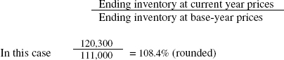
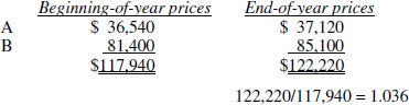
Thus, the base-year inventory layer is $100,000 (the end-of-year inventory stated at base-year cost). The second year requires the first index computation. Notice that in year 2 our extended totals are:
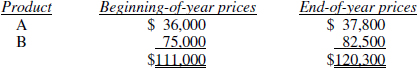
The year 2 index is 1.084 (120,300/111,000). This is the same as computed under the double-extension method because the beginning-of-the-year prices reflect the base-year price. This will not always be the case, as sometimes new items may be added to the pool, causing a change in the index. Thus, the cumulative index is the 1.084 current year index multiplied by the preceding year index of 1.00 to arrive at a link-chain index of 1.084.
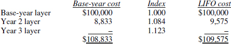
This index is then used to restate the inventory to base-year cost by dividing the inventory at end-of-year prices by the cumulative index: $120,300/1.084 = $111,000. The determination of the LIFO increment or decrement is then basically the same as the double-extension method. In year 2 the increment (layer) at base-year cost is $11,000 ($111,000 − 100,000). This layer must be valued at the prices effective when the layer was created, or extended at the cumulative index for that year. This results in an ending inventory at LIFO cost of:
The index for year 3 is computed as follows:
The next step is to determine the cumulative index which is the product of the preceding year's cumulative index and the current year index, or 1.123 (1.084 × 1.036). The new cumulative index is used to restate the inventory at end-of-year dollars to base-year cost. This is accomplished by dividing the end-of-year inventory by the new cumulative index. Thus, current inventory at base-year cost is $108,833 ($122,220 ÷ 1.123). In this instance we have experienced a decrement (a decrease from the prior year's $111,000). The determination of ending inventory is:
Finally, the same steps are performed for the year 4 computation. The current year index is 1.035 (133,900/129,380). The new cumulative index is 1.162 (1.035 × 1.123). The base-year cost of the current inventory is $115,232 (133,900/1.162). Thus, LIFO inventory at the end of year 4 is:
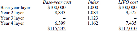
Notice how even though the numbers used were the same as those used in the double-extension example, the results were different (year 4 inventory under double-extension was $116,976)—however, not by a significant amount. It is much easier to keep track of beginning-of-the-year prices than base-year prices, but perhaps more importantly, it is easier to establish beginning-of-the-year prices for new items than to establish their base-year price. This latter reason is why the link-chain method is so much more desirable than the double-extension method. However, before electing or applying this method, a company must be able to establish a sufficient need as defined in the treasury regulations.
Indexing methods. Indexing methods can basically be broken down into two types: (1) an internal index and (2) an external index.
The internal index is merely a variation of the double-extension method. The regulations allow for the use of a statistically valid representative sample of the inventory to be double-extended. The index computed from the sample is then used to restate the inventory to base-year cost and to value the new layer.
The external index method, referred to in treasury regulations as the Inventory Price Index Computation (IPIC) Method, involves using indices published by the US Department of Labor's Bureau of Labor Statistics (BLS)2 and applying them to specified categories of inventory included in the taxpayer's LIFO pools. Taxpayers wanting to change to the IPIC Method from another LIFO method must obtain IRS consent by filing Form 3115, Application for Change in Accounting Method.
Alternative LIFO method for automobile dealers. A simplified dollar-value method is available for use by retail automobile dealers for valuing inventory of new automobiles and light-duty trucks. The use of this method and its acceptance for income tax purposes is conditioned on the application of several LIFO submethods, definitions and special rules. The reader is referred to Rev. Proc. 92-79 for a further discussion of this method.
LIFO accounting literature. GAAP for the application of LIFO has been based upon income tax rules rather than on financial accounting pronouncements. LIFO is cited in GAAP as an acceptable inventory method, but specific rules regarding its implementation are not provided. The income tax regulations, as discussed below, do provide specific rules for the implementation of LIFO and require financial statement conformity. For this reason, income tax rules have essentially defined the financial accounting treatment of LIFO inventories.
In recognition of the lack of authoritative accounting guidelines in the implementation of LIFO, the American Institute of Certified Public Accountants (AICPA)'s Accounting Standards Division formed a task force on LIFO inventory problems to prepare an Issues Paper on this topic. “Identification and Discussion of Certain Financial Accounting and Reporting Issues Concerning LIFO Inventories,” issued in 1984, identifies financial accounting issues resulting from the use of LIFO and includes advisory guidance on resolving them. Issues Papers, however, do not establish authoritative standards of financial accounting. The guidance provided by the task force is described below.3
- Specific goods versus dollar-value. Either the specific goods approach or dollar-value approach to LIFO is acceptable for financial reporting. Disclosure of whether the specific goods or dollar-value approach is used is not required.
- Pricing current year purchases. Three approaches to pricing LIFO inventory increments are available under income tax regulations—earliest acquisition price, latest acquisition price, and average acquisition price. The earliest acquisition price approach is the most compatible with financial reporting objectives, but all three are acceptable for financial reporting.
- Quantity to use to determine price. The price used to determine the inventory increment should be based on the cost of the quantity or dollars of the increment rather than on the cost of the quantity or dollars equal to the ending inventory. Disclosure of which approach is used is not required.
- Disclosure of LIFO reserve or replacement cost. The LIFO reserve or replacement cost and its basis for determination should be disclosed for financial reporting.
- Partial adoption of LIFO. If a company changes to LIFO, it should do so for all of its inventories. Partial adoption should only be allowed if there exists a valid business reason for not fully adopting LIFO. A planned gradual adoption of LIFO over several time periods is considered acceptable if valid business reasons exist (lessening the income statement effect of adoption in any one year is not a valid business reason). Where partial adoption of LIFO has been justified, the extent to which LIFO has been adopted should be disclosed. This can be disclosed by indicating either the portion of the ending inventory priced on LIFO or the portion of cost of sales resulting from LIFO inventories.
- Methods of pooling. An entity should have valid business reasons for establishing its LIFO pools. Additionally, the existence of a separate legal entity that has no economic substance is not reason enough to justify separate pools. Disclosure of details regarding an entity's pooling arrangements is not required.
- New items entering a pool. New items should be added to a pool based on what the items would have cost had they been acquired in the base period (reconstructed cost) rather than based on their current cost. The reconstructed cost should be determined based on the most objective sources available, including published vendor price lists, vendor quotes, and general industry indexes. Where necessary, the use of a substitute base year in making the LIFO computation is acceptable. Disclosure of the way that new items are priced is not required.
- Dollar-value index. The required index can be developed using two possible approaches, the unit cost method or the cost component method. The unit cost method measures changes in the index based on the weighted-average increase or decrease in the unit costs of raw materials, work in process, and finished goods inventory. The cost component method, on the other hand, measures changes in the index by the weighted-average increase or decrease in the component costs of material, labor, and overhead that make up ending inventory. Either of these methods is acceptable.
- LIFO liquidations. The effects on income of LIFO inventory liquidations should be disclosed in the notes to the financial statements. A replacement reserve for the liquidation should not be provided. When an involuntary LIFO liquidation occurs, the effect on income of the liquidation should not be deferred.
When a LIFO liquidation occurs, there are three possible ways to measure its effect on income:
- The difference between actual cost of sales and what cost of sales would have been had the inventory been reinstated under the entity's normal pricing procedure
- The difference between actual cost of sales and what cost of sales would have been had the inventory been reinstated at year-end replacement cost
- The amount of the LIFO reserve at the beginning of the year which was credited to income (excluding the increase in the reserve due to current year price changes)
The first method is considered preferable. Disclosure of the effect of the liquidation should give effect only to pools with decrements (i.e., there should be no netting of pools with decrements against other pools with increments).
- Lower of cost or market. The most reasonable approach to applying the lower of cost or market rules to LIFO inventory is to base the determination on groups of inventory rather than on an item-by-item approach. A pool constitutes a reasonable grouping for this purpose. An item-by-item approach is permitted by authoritative accounting literature, particularly for obsolete or discontinued items.
For companies with more than one LIFO pool, it is permissible to aggregate the pools in applying the lower of cost or market test if the pools are similar. Where the pools are significantly dissimilar, aggregating the pools is not appropriate.
Previous write-downs to market value of the cost of LIFO inventories should be reversed after a company disposes of the physical units of the inventory for which reserves were provided. The reserves at the end of the year should be based on a new computation of cost or market.
- LIFO conformity and supplemental disclosures. A company may present supplemental non-LIFO disclosures within the historical cost framework. If nondiscretionary variable expenses (i.e., profit sharing based on earnings) would have been different based on the supplemental information, then the company should give effect to such changes. Additionally, the supplemental disclosure should reflect the same type of income tax effects as required by generally accepted accounting principles in the primary financial statements.
A company may use different LIFO applications for financial reporting than it uses for income tax purposes. Any such differences should be accounted for as temporary differences with the exception of differences in the allocation of cost to inventory in a business combination. Any differences between LIFO applications used for financial reporting and those used for income tax purposes need not be disclosed beyond the requirements of ASC 740.
- Interim reporting and LIFO. The Task Force's conclusions on interim reporting of LIFO inventory are discussed in the chapter on interim reporting.
- Different financial and income tax years. A company with different fiscal year-ends for financial reporting and income tax reporting should make a separate LIFO calculation for financial purposes using its financial reporting year as a discrete period for that calculation.
- Business combinations accounted for by the purchase method. Inventory acquired in a business combination accounted for by the purchase method will be recorded at fair value at the date of the combination. The acquired company may be able to carry over its prior basis for that inventory for income tax purposes, causing a difference between GAAP and income tax basis. An adjustment should be made to the fair value of the inventory only if it is reasonably estimated that it will be liquidated in the future. The adjustment would be for the income tax effect of the difference between income tax and GAAP basis.
Inventory acquired in such a combination should be considered the LIFO base inventory if the inventory is treated by the company as a separate business unit or a separate LIFO pool. If instead the acquired inventory is combined into an existing pool, then the acquired inventory should be considered as part of the current year's purchases.
- Changes in LIFO applications. A change in a LIFO application is a change in accounting principle. LIFO applications refer to the approach (i.e., dollar value or specific goods), computational technique, or the numbers or contents of the pools.
ASC 810-10-55 provides guidance for intercompany transfers. The focus of this section is the LIFO liquidation effect caused by transferring inventories, which in turn creates intercompany profits. This liquidation can occur when (1) two components of the same taxable entity transfer inventory, for example, when a LIFO method component transfers inventory to a non-LIFO component, or (2) when two separate taxable entities that consolidate transfer inventory, even though both use the LIFO method.
This LIFO liquidation creates profit that must be eliminated along with other intercompany profits.
LIFO income tax rules and restrictions. As discussed previously, most of the rules and regulations governing LIFO originate in the US IRC and the related regulations, revenue rules, revenue procedures, and judicial decisions. Taxpayers electing to use the LIFO inventory method are subject to myriad rules and restrictions, such as:
- The inventory is to be valued at cost regardless of market value (i.e., application of the lower of cost or market rule is not allowed).
- Changes in the LIFO reserve can potentially cause the taxpayer to be subject to alternative minimum tax (AMT) or increase the amount of AMT.
- Corporations that use the LIFO method whose stockholders subsequently elect to be taxed as an “S” Corporation are required to report as income their entire LIFO reserve resulting in a special tax under IRC §1363(d) that is payable in four annual installments. The “S” Corporation is, however, permitted to retain LIFO as its inventory accounting method after the election.
- Once elected, the LIFO method must continue to be used consistently in future periods. A taxpayer is permitted, subject to certain restrictions, to revoke its LIFO election in accordance with Rev. Proc. 99-49. After revocation however, the taxpayer is precluded from reelecting LIFO for a period of five taxable years beginning with the year of the change. For GAAP purposes, a change to or from the LIFO method is accounted for as a change in accounting principle under ASC 250.
A unique rule regarding LIFO inventories is referred to as the LIFO Conformity Rule. A taxpayer may not use a different inventory method in reporting profit or loss of the entity for external financial reports. Thus, if LIFO is elected for income tax purposes, it must also be used for accounting purposes.
Treasury regulations permit certain exceptions to this general rule. Among the exceptions allowable under the regulations are the following:
- The use of an inventory method other than LIFO in presenting information reported as a supplement to or explanation of the taxpayer's primary presentation of income in financial reports to outside parties. (Reg. §1.472-2[e][1][i])
- The use of an inventory method other than LIFO to determine the value of the taxpayer's inventory for purposes of reporting the value of such inventory as an asset on the statement of financial position. (Reg. §1.472-2[e][1][ii])
- The use of an inventory method other than LIFO for purposes of determining information reported in internal management reports. (Reg. §1.472-2[e][1][iii])
- The use of an inventory method other than LIFO for financial reports covering a period of less than one year. (Reg. §1.472- 2[e][1][iv])
- The use of lower of LIFO cost or market to value inventories for financial statements while using LIFO cost for income tax purposes. (Reg. §1.472-2[e][1][v])
- For inventories acquired by a corporation in exchange for issuing stock to a stockholder that, immediately after the exchange, is considered to have control (a section 351 transaction), the use of the transferor's acquisition dates and costs for GAAP while using redetermined LIFO layers for tax purposes. (Reg. §1.472-2[e][1][vii])
- The inclusion of certain costs (under full absorption) in inventory for income tax purposes, as required by regulations, while not including those same costs in inventory under GAAP (full absorption). (Reg. §1.472-2[e][8][i])
- The use of different methods of establishing pools for GAAP purposes and income tax purposes. (Reg. §1.472-2[e][8][ii])
- The use of different determinations of the time sales or purchases are accrued for GAAP purposes and tax purposes. (Reg. §1.472-2[e][8][xii])
- In the case of a business combination, the use of different methods to allocate basis for GAAP purposes and income tax purposes. (Reg. §1.472-29[e][8][xiii])
Another important consideration in applying the LIFO conformity rule is the law concerning related corporations. In accordance with the Tax Reform Act of 1984, all members of the same group of financially related corporations are treated as a single taxpayer when applying the conformity rule. Previously, taxpayers were able to circumvent the conformity rule by having a subsidiary on LIFO, while the non-LIFO parent presented combined non-LIFO financial statements. This is a violation of the conformity requirement [Sec. 472(g)].
The LIFO conformity rule is viewed as a major obstacle to the adoption of International Financial Reporting Standards (IFRS) in the United States. Since IFRS does not permit the use of LIFO for valuing inventories, should a US taxpayer convert from US GAAP to IFRS in presenting its basic financial statements, that taxpayer would violate the LIFO conformity rule, which would result in an automatic revocation of the LIFO election. Thus, the adoption of IFRS would likely cause a heavy income tax burden for those taxpayers using LIFO to value their inventories.
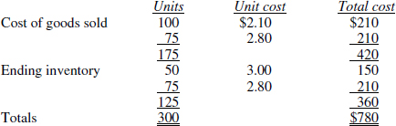
Weighted-average and moving-average.
Another method of inventory valuation involves averaging and is commonly referred to as the weighted-average method.
Under this method the cost of goods available for sale (beginning inventory plus net purchases) is divided by the number of units available for sale to obtain a weighted-average cost per unit. Ending inventory and cost of goods sold are then priced at this average cost.
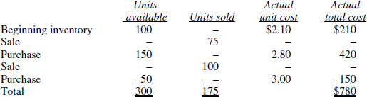
Assume the following data:
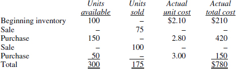
The weighted-average cost per unit is $780/300, or $2.60. Ending inventory is 125 units (300 − 175) at $2.60, or $325; cost of goods sold is 175 units at $2.60, or $455.
When the weighted-average assumption is applied using a perpetual inventory system, the average cost is recomputed after each purchase. This process is referred to as a moving average. Cost of goods sold is recorded using the most recent average. This combination is called the moving-average method and is applied below to the same data used in the weighted-average example above.
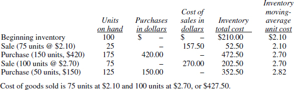
Cost of goods sold is 75 units at $2.10 and 100 units at $2.70, or $427.50.
This method is permitted for financial reporting purposes but had historically been prohibited for income tax purposes (Rev. Ruling 71-234). The IRS has issued Revenue Procedure 2008-43, which grants limited use of this method for income tax reporting purposes. This relief is only available to taxpayers that were already using an average cost method for financial reporting purposes. In addition, an electing taxpayer is required to meet both of the following safe harbors:
- The taxpayer must recompute the rolling average inventory price with every new purchase, or no less frequently than monthly.
- The results under the rolling average method may not vary by more than 1% from the results using a FIFO or specific identification method. A shortcut method is permitted to be used to meet this safe harbor. If the taxpayer's annual turnover for its entire inventory exceeds four times, this safe harbor is considered to have been met.
Comparison of cost flow assumptions.
Of the three cost flow assumptions, FIFO and LIFO produce the most extreme results, while results from using the weighted-average method generally fall somewhere in between. The selection of one of these methods involves a detailed analysis of the organization's objectives, industry practices, current and expected future economic conditions, and most importantly, the needs of the intended users of the financial statements.
The following table compares the relative effects of using FIFO and LIFO cost assumptions on the statement of financial position and statement of income under differing economic conditions:
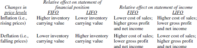
In periods of rising prices, the LIFO method is generally thought to best fulfill the objective of providing the clearest measure of periodic net income. It does not, however, provide an accurate estimate of inventory cost in an inflationary environment. However, this shortcoming can usually be overcome by providing additional disclosures in the notes to the financial statements. In periods of rising prices, a prudent business should use the LIFO method because it will result in a decrease in the current income tax liability when compared to other alternatives. In a deflationary period, the opposite is true.
FIFO is a balance-sheet-oriented costing method. It gives the most accurate estimate of the current cost of inventory during periods of changing prices. In periods of rising prices, the FIFO method will result in higher income taxes than the other alternatives, while in a deflationary period FIFO provides for a lesser income tax burden. However, a major advantage of the FIFO method is that it is not subject to all of the complex regulations and requirements of the income tax code that govern the use of LIFO.
The average methods do not provide an estimate of current cost information on either the statement of financial position or income statement. The average methods are not permitted to be used for income tax purposes and therefore, their use for financial reporting purposes would necessitate the use of FIFO for income tax reporting purposes since LIFO requires financial statement conformity.
Although price trends and underlying objectives are important to consider in selecting a cost flow assumption, other considerations are the risk of experiencing unintended liquidations of LIFO layers, as well as the effects of the chosen method on cash flow, capital maintenance, collateral requirements, and restrictive covenants imposed by lenders, etc.
Lower of Cost or Market (LCM)
As stated in ASC 330-10-20:
...as used in the phrase lower of cost or market, the term market means current replacement cost, provided that it meets both the following conditions: a) market shall not exceed the net realizable value, and b) market shall not be less than net realizable value reduced by an allowance for an approximately normal profit margin.
Inventory can lose value for a variety of reasons including damage, spoilage, obsolescence, changes in market prices, and the like. The application of LCM is a means of attempting to measure loss of value and recognize the effects in the period in which this occurs.
The term “market” means current replacement cost not to exceed a ceiling of net realizable value (selling price less reasonably estimable costs of completion and disposal) or be less than a floor of net realizable value adjusted for a normal profit margin.
LCM is not applied in conjunction with the LIFO method of inventory valuation for income tax purposes. However, it is important to note that LCM/LIFO is applied for financial reporting purposes. Such application gives rise to a temporary difference in the carrying value of inventory between financial statements and income tax returns. LCM/LIFO for financial reporting was discussed earlier in this chapter.
LCM may be applied to either the entire inventory or to each individual inventory item. The primary objective for selecting between the alternative methods of applying the LCM rule is to select the one that most clearly reflects periodic income. The rule is most commonly applied to the inventory on an item-by-item basis. The reason for this application is twofold.
- It is required by income tax purposes unless it involves practical difficulties, and
- It provides the most conservative valuation of inventories, because decreases in the value of one item are not offset by increases in the value of another.
The application of these principles is illustrated in this example. Assume the following information for products A, B, C, D, and E:
First, determine the market value and then compare this to historical cost. Market value is equal to the replacement cost, but cannot exceed the net realizable value (NRV) nor be below net realizable value less the normal profit percentage.
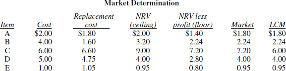
NRV (ceiling) equals selling price less costs of completion (e.g., item A: $2.50 − .50 = $2.00). NRV less profit (floor) is self-descriptive (e.g., item A: $2.50 − .50 − .60 = $1.40). Market is replacement cost unless lower than the floor or higher than the ceiling. Note that market must be designated before LCM is determined. Finally, LCM is the lower of cost or market value.
Replacement cost is a valid measure of the future utility of the inventory item, since increases or decreases in the enterprise's purchase price generally foreshadow related increases or decreases in the price at which it is able to sell the item. The ceiling and the floor provide safeguards against the recognition of either excessive profits or excessive losses in future periods in those instances where the selling price and replacement cost do not move in the same direction in a proportional manner. The ceiling avoids the recognition of additional losses in the future when the selling price is falling faster than replacement cost. Without the ceiling constraint, inventories would be carried at an amount in excess of their net realizable value. The floor avoids the recognition of abnormal profits in the future when replacement cost is falling faster than the selling price. Without the floor, inventories would be carried at a value less than their net realizable value minus a normal profit.
The loss from writing inventories down to LCM is generally reflected on the income statement in cost of goods sold. If material, the loss must be separately captioned in the income statement. While GAAP is not explicit as to presentation, it would appear that this adjustment could either be displayed as a separately identified charge within cost of goods sold, or as an administrative expense. The write-down is recorded as a debit to a loss account and a credit either to an inventory or a valuation allowance account.
Inventory estimation methods.
There are instances in which an accountant must estimate the value of inventories without an actual physical count. Some of the estimation methods used to accomplish this are the retail method, the LIFO retail method, and the gross profit method. These methods are not cost flow assumptions like LIFO and FIFO; rather, they are computational methods that have been devised to assist in estimating inventory cost under the relevant cost flow assumption.
Retail method. The retail method is used by retailers to estimate the cost of their ending inventory. The retailer can either take a physical inventory at retail prices or estimate ending retail inventory and then use a computed cost-to-retail ratio to convert the ending inventory priced at retail to its estimated cost. This method eliminates the process of going back to original vendor invoices or other documents in order to determine the original cost for each inventoriable item. The retail method can be used under any of the three cost flow assumptions discussed earlier: FIFO, LIFO, or average cost. As with ordinary FIFO or average cost, the LCM rule is also applied when either one of these two cost assumptions is used in conjunction with the retail method.
The key to applying the retail method is determining the cost-to-retail ratio. The calculation of this ratio varies depending upon the cost flow assumption selected. The cost-to-retail ratio provides a measure of the relationship between the cost of goods available for sale and the retail price of these same goods. This ratio is used to convert the ending retail inventory back to cost. The computation of the cost-to-retail ratio for the FIFO and average cost methods is described below. The use of the LIFO cost flow assumption with this method is discussed in the succeeding section.
- FIFO cost—The FIFO method assumes that the ending inventory is made up of the latest purchases. Therefore, beginning inventory is excluded from the computation of the cost-to-retail ratio, and the computation uses the cost of current year net purchases divided by their retail value adjusted for both net markups and net markdowns as will be further explained and illustrated.
- FIFO (LCM)—The computation is basically the same as FIFO cost, except that markdowns are excluded from the computation of the cost-to-retail ratio.
- Average cost—Average cost assumes that ending inventory consists of all goods available for sale. Therefore, the cost-to-retail ratio is computed by dividing the cost of goods available for sale (Beginning inventory + Net purchases) by the retail value of these goods adjusted for both net markups and net markdowns.
- Average cost (LCM)—Is computed in the same manner as average cost, except that markdowns are excluded from the calculation of the cost-to-retail ratio.
A simple example illustrates the computation of the cost-to-retail ratio under both the FIFO cost and average cost methods in a situation where no markups or markdowns exist.
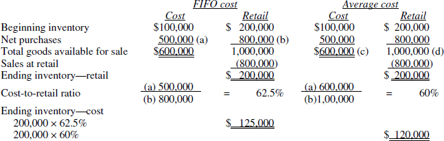
Note that the only difference in the two examples is the numbers used to calculate the cost-to-retail ratio.
The lower of cost or market aspect of the retail method is a result of the treatment of net markups and net markdowns. Net markups (markups less markup cancellations) are net increases above the original retail price, which are generally caused by changes in supply and demand. Net markdowns (markdowns less markdown cancellations) are net decreases below the original retail price. An approximation of “lower of cost or market” pricing is achieved by including net markups but excluding net markdowns, from the cost-to-retail ratio.
To understand this approximation, assume a toy is purchased for $6, and the retail price is set at $10. It is later marked down to $8. A cost-to-retail ratio including markdowns would be $6 divided by $8 or 75%, and ending inventory would be valued at $8 times 75%, or $6 (original cost). The logic behind including markdowns in the cost-to-retail ratio is the assumption that these inventories would eventually be marked down and that markdowns are a normal part of business for this enterprise and/or these types of inventories. A cost-to-retail ratio excluding markdowns would be $6 divided by $10 or 60%, and ending inventory would be valued at $8 times 60%, or $4.80 (LCM). The logic behind excluding markdowns from the cost-to-retail ratio is that the enterprise did not expect to mark these inventory items down and that this is not a normal occurrence. The write-down to $4.80 reflects the loss in utility which is evidenced by the reduced retail price.
The application of the lower of cost or market rule is illustrated for both the FIFO and average cost methods in the example below. Remember, if the markups and markdowns below had been included in the previous example, both would have been included in the cost-to-retail ratio.
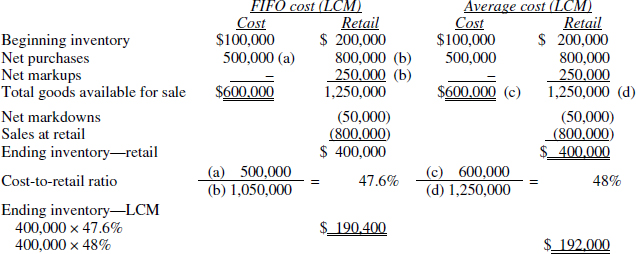
Under the FIFO (LCM) method all of the markups are considered attributable to the current period purchases. While this is not necessarily accurate, it provides the most conservative estimate of the ending inventory.
There are a number of additional issues that affect the computation of the cost-to-retail ratio. Purchase discounts and freight-in affect only the cost column in this computation. The sales figure that is subtracted from the adjusted cost of goods available for sale in the retail column must be gross sales after adjustment for sales returns. Sales discounts are not included in the computation. If sales are recorded gross, then deduct the gross sales figure. If sales are recorded net, then both the recorded sales and sales discount must be deducted to give the same effect as deducting gross sales. Normal spoilage is generally allowed for in the enterprise's pricing policies, and for this reason it is deducted from the retail column after the calculation of the cost-to-retail ratio. Abnormal spoilage, on the other hand, is deducted from both the cost and retail columns before the cost-to-retail calculation as it could otherwise distort the ratio. It is then generally reported as a separate loss, either within cost of goods sold or administrative expenses. Abnormal spoilage generally arises from a major theft or casualty, while normal spoilage is usually due to shrinkage or breakage. These determinations and their treatments will vary depending upon the enterprise's policies.
When applying the retail method, separate computations are made for any departments that experience significantly higher or lower gross profit margins. Distortions arise in applying the retail method when a department sells goods with gross profit margins that vary in a proportion different from the gross profit margins of goods purchased during the period. In this case, the cost-to-retail percentage would not be representative of the mix of goods in ending inventory. Also, manipulations of income are possible by planning the timing of markups and markdowns.
The retail method is an acceptable method of estimating inventories under FIFO (LCM) for income tax purposes. Income tax regulations require valuation at lower of cost or market (except for LIFO) and regular and consistent physical counts of inventory at each location.
LIFO retail method. As with other LIFO methods, treasury regulations are the governing force behind the LIFO retail method. The regulations differentiate between a “variety” store, which is required to use an internally computed index, and a “department” store, which is permitted to use a price index published by the Bureau of Labor Statistics. The computation of an internal index was previously discussed in the dollar-value LIFO section. It involves applying the double-extension method to a representative sample of the ending inventory. Selection of an externally published index is to be in accordance with the treasury regulations.
The steps used in computing the value of ending inventory under the LIFO retail method are listed below and then applied in an example for illustrative purposes.
- Calculate (or select) the current year conversion price index. Recall that in the base year this index will be 1.00.
- Calculate the value of the ending inventory at both cost and retail. Remember, as with other LIFO methods, income tax regulations do not permit the use of LCM, so both markups and markdowns are included in the computation of the cost-to-retail ratio. However, the beginning inventory is excluded from goods available for sale at cost and at retail.
- Restate the ending inventory at retail to base-year retail. Divide the current ending inventory at retail by the current year index determined in Step 1.
- Layers are then treated as they were for the dollar-value LIFO example presented earlier. If the ending inventory restated to base-year retail exceeds the previous year's amount at base-year retail, a new layer is established.
- The computation of LIFO cost is the last step and requires multiplying each layer at base-year retail by the appropriate price index and multiplying this product by the cost-to-retail ratio in order to arrive at the LIFO cost for each layer.
The following example illustrates a two-year period to which the LIFO retail method is applied. The first period represents the first year of operations for the company and is its base year.
Year 1
Step 1—Because this is the base year, there is no need to compute an index, as it will always be 1.00.
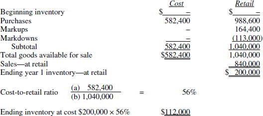
Step 3—Because this is the base year, the restatement to base-year cost is not necessary; however, the computation would be $200,000/1.00 = $200,000.
Steps 4 and 5—The determination of layers is again unnecessary in the base year; however, the computation would take the following format:
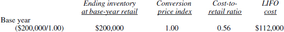
Year 2
Step 1—We make the assumption that the computation of an internal index yields a result of 1.12 (obtained by double-extending a representative sample).
Step 2—
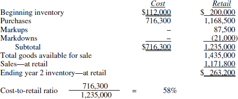
Step 3—The restatement of ending inventory at current year retail to base-year retail is done using the index computed in Step 1. In this case it is $263,200/1.12 = $235,000.
Steps 4 and 5—There is a LIFO layer in year 2 because the $235,000 inventory at base-year retail exceeds the year 1 amount of $200,000.
The computation of the LIFO cost for each layer is shown below.

The treatment of subsequent increments and decrements is the same for this method as it is for the regular dollar-value method.
Gross profit method. The gross profit method is used to estimate ending inventory when a physical count is not taken. It can also be used to evaluate the reasonableness of a given inventory amount. Assume the following data:
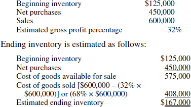
The gross profit method is used for interim reporting estimates, for conducting analytical review procedures by independent accountants in audits and review engagements, and for estimating inventory lost in fires or other catastrophes. The method is not acceptable, however, for either income tax or annual financial reporting purposes.
Standard costs. Standard costs are predetermined unit costs used by manufacturing firms for planning and control purposes. Standard costs are often used to develop approximations of GAAP inventories for financial reporting purposes. The use of standard cost approximations in financial reporting is acceptable only if adjustments to the standards are made periodically to reflect current conditions and if their use approximates the results that would be obtained by directly applying one of the recognized cost flow assumptions.
The Bavarian Clock Company (BCC) uses standard costing to value its FIFO inventory. One of its products is the Men's Chronometer wristwatch, for which the following bill of materials has been constructed:
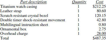
The industrial engineering department designed the following labor routing for assembly of the Men's Chronometer and determined the standard process times:
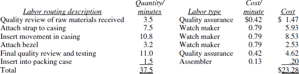
Thus, the total standard cost of the Men's Chronometer is $510.63 ($487.35 material and overhead cost + $23.28 labor cost). At the beginning of December, there are 1,087 Men's Chronometers in finished goods inventory, which are recorded at standard cost, resulting in a beginning inventory valuation of $555,054.81 (= $510.63 × 1,087 units).
During December, BCC records actual material costs of $1,915,312.19, actual labor costs of $111,844.40, and actual overhead costs of $124,831.55 related to the Men's Chronometer, which are charged to the inventory account. During the month, BCC manufactures 4,105 Men's Chronometers and ships 4,385, leaving 807 units in finished goods inventory. At a standard cost of $510.63 per unit, this results in a month-end finished goods inventory balance of $412,078.41. The monthly charge to cost of goods sold is calculated as follows:
At month-end, the purchasing manager conducts his quarterly review of the bill of materials and determines that the cost of the bezel has permanently increased by $4.82, bringing the total standard bezel cost to $124.97 and therefore the total standard cost of the Men's Chronometer to $515.45. This increases the value of the ending inventory by $3,889.74 ($4.82 standard cost increase × 807 units in finished goods inventory), to $415,968.15, while reducing the cost of goods sold to $2,291,074.80. The following entry records the month-end inventory valuation at standard cost:
![]()
As a cross-check, BCC's controller divides the cost of goods sold by the total number of units shipped, and arrives at an actual unit cost of $522.48, as opposed to the standard costs of $515.45. The variance from the standard cost is $7.03 per unit, or a total of $30,826.55. Upon further investigation, she finds that overnight delivery charges of $1,825 were incurred for a shipment of watch casings, while there was a temporary increase in the cost of the leather strap of $2.83 for a 1,000-unit purchase, resulting in an additional charge of $2,830. She elects to separately track these excess material-related costs with the following entry:
![]()
In addition, the production staff incurred overtime charges of $16,280 during the month. Since overtime is not included in the labor routing standard costs, the controller separately tracks this information with the following entry:
![]()
Finally, the controller determines that some costs comprising the overhead cost pool exceeded the budgeted overhead cost during the month, resulting in an excess charge of $9,891.55 to the Men's Chronometer cost of goods sold. She separates this expense from the cost of goods sold with the following entry:
![]()
Her variance analysis has identified all causes of the $30,826.55 cost overage, as noted in the following table:
As explained previously, variances resulting from abnormal costs incurred are considered period costs and, thus, are not allocated to inventory.
Other inventory valuation methods.
Base stock. The base stock method assumes that a certain level of inventory investment is necessary for normal business activities and is, therefore, permanent. The base stock inventory is carried at historical cost. Decreases in the base stock are considered temporary and are charged to cost of goods sold at replacement cost. Increases are carried at current year costs. The base stock approach is seldom used in practice, since it is not allowed for income tax purposes, and the LIFO method yields similar results.
Direct costing. An alternative to full absorption costing is direct costing. Direct costing (also referred to as variable costing) requires classifying only direct materials, direct labor, and variable production overhead as inventory costs. Under this method, all fixed costs are accounted for as period costs. The exclusion of all overhead from inventory costs is not an acceptable accounting method for GAAP or under the US Treasury Regulations for income tax purposes.
Relative sales value. Relative sales (or net realizable) values are used to assign costs to inventory items purchased or manufactured in groups. This method is applicable to joint products, subdivided assets such as real estate lots, and basket purchases.
For example, products A and B have the same processes performed on them up to the split-off point. The total cost incurred to this point is $80,000. This cost can be assigned to products A and B using their relative sales value at the split-off point. If A could be sold for $60,000 and B for $40,000, the total sales value is $100,000. The cost would be assigned on the basis of each product's relative sales value. Thus, A would be assigned a cost of $48,000 (60,000/100,000 × 80,000) and B a cost of $32,000 (40,000/100,000 × 80,000).
Differences between GAAP and Income Tax Accounting for Inventories
Full absorption costing—income tax.
Prior to the Tax Reform Act of 1986 (TRA 1986), production costing for GAAP and for income tax purposes were very similar. However, TRA 1986 included provisions referred to as Uniform Capitalization (UNICAP), which changed inventory costing for income tax purposes by requiring certain additional indirect costs that are not capitalizable under GAAP be capitalized rather than expensed for income tax purposes. TRA 1986 requires that manufacturers capitalize rather than expense these additional items:
- Depreciation and amortization in excess of that reported in financial statements
- Percentage depletion in excess of cost
- Rework labor, scrap, and spoilage costs
- Allocable general and administrative costs related to the production function.
For income tax purposes, these costs, as well as the indirect production costs listed above for inventory costing under GAAP, are allocated to the WIP and finished goods inventories. Examples of general and administrative costs that must be allocated include payroll department costs, wages of security guards, and the president's salary. The difference between the GAAP and income tax inventory carrying values is a temporary difference, which requires deferred income tax accounting (discussed in Chapter 24).
Uniform capitalization rules—income tax versus GAAP.
TRA 1986 established the UNICAP rules for inventory costs for tax purposes. ASC 330-10-55 states that capitalizing a cost for income tax purposes does not, by itself, indicate that it is preferable or even appropriate to capitalize the cost for financial reporting purposes. Although a cost may be required to be capitalized for income tax purposes, management must analyze the individual facts and circumstances based on the nature of its operations and industry practice to determine whether to capitalize the cost for financial reporting purposes.
Inventory capitalization for retailers/wholesalers—income tax versus GAAP.
Prior to TRA 1986, retailers and wholesalers recorded their inventory as the invoice price plus the cost of applicable sales tax and freight-in under both GAAP and income tax law. TRA 1986 applied UNICAP to certain retailers and wholesalers and introduced a requirement that additional costs be capitalized. Inventories of retailers/wholesalers whose average annual gross receipts for the preceding three years are $10 million or less are exempt from applying UNICAP.
The costs which must be capitalized have been divided into two categories. The first category is direct costs and includes the inventory invoice price plus transportation. Also included in direct costs is the cost of labor for purchasing, storing, and handling inventory items. The second category is indirect costs and consists of any costs that directly benefit or are incurred because of the performance of a resale activity. The following types of indirect costs must be capitalized under UNICAP:
- Off-site storage or warehousing
- Purchasing
- Handling, processing, assembly, and repackaging
- Allocable general and administrative costs related to the above three functions.
The indirect costs are allocated between inventory and cost of goods sold by using traditional methods (specific identification, standard costing methods, etc.) or one of three simplified methods. Temporary differences require deferred income tax accounting as discussed in the chapter on ASC 740, Income Taxes.
Other Inventory Topics
Purchase commitments.
Purchase commitments generally are not recognized in the financial statements because they are executory in nature. However, disclosure in the notes to the financial statements is required for firm purchase commitments that are material in amount.
If at the date of a statement of financial position the contract price of these commitments exceeds the market value, the estimated loss is accrued and reported as a loss in the income statement. This results in recognition of the loss before the inventory is actually purchased.
Inventories valued at selling price.
In exceptional cases, inventories may be reported at sales price less estimated disposal costs. Such treatment is justified when cost is difficult to determine, quoted market prices are available, marketability is assured, and units are interchangeable. Precious metals, certain agricultural products, and meat are examples of inventories valued in this manner. When inventory is valued above cost, revenue is recognized before the time of sale. Naturally full disclosure in the financial statements is required.
Stripping costs incurred during production in the mining industry.
ASC 930-330 states that stripping costs incurred during a mine's production phase are to be accounted for as variable production costs and therefore allocated to inventory. The ASC is limited to stripping costs incurred during the period when inventory is being produced (i.e., extracted) and did not address the accounting for these costs when incurred during the preproduction phase of the mine.
Interim reporting.
The principles used to determine ending inventory and cost of goods sold in annual reports are also used in interim reports, although four exceptions are allowed (under ASC 270). These are
- The gross profit method may be used to estimate cost of goods sold and ending inventory.
- When LIFO layers are liquidated during the interim period but are expected to be replaced by year-end, cost of goods sold is adjusted to reflect current costs rather than older LIFO costs.
- Temporary market declines need not be recognized if substantial evidence exists that market prices will recover. If LCM losses are recorded in one or more interim periods and are recovered by year-end, the recovery is recognized as a fourth-quarter gain.
- Planned standard cost variances expected to reverse by year-end are not recognized.
See a complete discussion of interim financial reporting see the chapter on ASC 270.
1 This guidance does not apply to arrangements accounted for as derivatives under ASC 815, or to exchanges of software or real estate.
2 For more information see http://www.bls.gov
3 The issues paper can be found at tinyurl.com/8j3f8t7.