Key Topics

Today we review basic routing concepts, including exactly how a packet is processed by intermediary devices (routers) on its way from source to decision. We then review the basic routing methods, including connected, static, and dynamic routes. Because dynamic routing is such a large CCNA topic area, we spend some time discussing classifications as well as the basic features of distance vector and link-state routing protocols.

Packet Forwarding

Packet forwarding by routers is accomplished through path determination and switching functions. The path determination function is the process of how the router determines which path to use when forwarding a packet. To determine the best path, the router searches its routing table for a network address that matches the packet’s destination IP address.

One of three path determinations results from this search:

  Directly connected network: If the destination IP address of the packet belongs to a device on a network that is directly connected to one of the router’s interfaces, that packet is forwarded directly to that device. This means that the destination IP address of the packet is a host address on the same network as this router’s interface.

  Remote network: If the destination IP address of the packet belongs to a remote network, the packet is forwarded to another router. Remote networks can be reached only by forwarding packets to another router.

  No route determined: If the destination IP address of the packet does not belong to either a connected or remote network, and the router does not have a default route, the packet is discarded. The router sends an Internet Control Message Protocol (ICMP) Unreachable message to the source IP address of the packet.

In the first two results, the router completes the process by switching the packet out the correct interface. It does this by reencapsulating the IP packet into the appropriate Layer 2 data-link frame format for the exit interface. The type of Layer 2 encapsulation is determined by the type of interface. For example, if the exit interface is Fast Ethernet, the packet is encapsulated in an Ethernet frame. If the exit interface is a serial interface configured for PPP, the IP packet is encapsulated in a PPP frame.

Path Determination and Switching Function Example

Most of the study resources have detailed examples with excellent graphics that explain the path determination and switching functions performed by routers as a packet travels from source to destination.

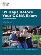
Although we do not have an abundance of room here to repeat those graphics, we can textually review an example using one graphic, shown in Figure 18-1.

For brevity, only the last two octets of the MAC address are shown in the figure.

1. PC1 has a packet to be sent to PC2.

   Using the AND operation on the destination’s IP address and PC1’s subnet mask, PC1 has determined that the IP source and IP destination addresses are on different networks. Therefore, PC1 checks its Address Resolution Protocol (ARP) table for the IP address of the default gateway and its associated MAC address. It then encapsulates the packet in an Ethernet header and forwards it to R1.

2. Router R1 receives the Ethernet frame.

   Router R1 examines the destination MAC address, which matches the MAC address of the receiving interface, FastEthernet 0/0. R1 will therefore copy the frame into its buffer.

   R1 decapsulates the Ethernet frame and reads the destination IP address. Because it does not match any of R1’s directly connected networks, the router consults its routing table to route this packet.

   R1 searches the routing table for a network address and subnet mask that would include this packet’s destination IP address as a host address on that network. The entry with the longest match (longest prefix) is selected. R1 then encapsulates the packet in the appropriate frame format for the exit interface and switches the frame to the interface (FastEthernet 0/1 in our example). The interface then forwards it to the next hop.

3. Packet arrives at Router R2.

   R2 performs the same functions as R1, except this time the exit interface is a serial interface—not Ethernet. Therefore, R2 encapsulates the packet in the appropriate frame format used by the serial interface and sends it to R3. For our example, assume the interface is using High-Level Data Link Control (HDLC), which uses the data-link address 0x8F. Remember, there are no MAC addresses on serial interfaces.

4. Packet arrives at R3.

   R3 decapsulates the data-link HDLC frame. The search of the routing table results in a network that is one of R3’s directly connected networks. Because the exit interface is a directly connected Ethernet network, R3 needs to resolve the destination IP address of the packet with a destination MAC address.

   R3 searches for the packet’s destination IP address of 192.168.4.10 in its ARP cache. If the entry is not in the ARP cache, R3 sends an ARP request out its FastEthernet 0/0 interface.

   PC2 sends back an ARP reply with its MAC address. R3 updates its ARP cache with an entry for 192.168.4.10 and the MAC address returned in the ARP reply.

   The IP packet is encapsulated into a new data-link Ethernet frame and sent out R3’s FastEthernet 0/0 interface.

5. Ethernet frame with encapsulated IP packet arrives at PC2.

   PC2 examines the destination MAC address, which matches the MAC address of the receiving interface—that is, its own Ethernet NIC. PC2 will therefore copy the rest of the frame. PC2 sees that the Ethernet Type field is 0x800, which means that the Ethernet frame contains an IP packet in the data portion of the frame. PC2 decapsulates the Ethernet frame and passes the IP packet to its operating system’s IP process.

Routing Methods

A router can learn routes from three basic sources:

  Directly connected routes: Automatically entered in the routing table when an interface is activated with an IP address

  Static routes: Manually configured by the network administrator and are entered in the routing table if the exit interface for the static route is active

  Dynamic routes: Learned by the routers through sharing routes with other routers that use the same routing protocol.

In many cases, the complexity of the network topology, the number of networks, and the need for the network to automatically adjust to changes require the use of a dynamic routing protocol. Dynamic routing certainly has several advantages over static routing; however, static routing is still used in networks today. In fact, networks typically use a combination of both static and dynamic routing.

Table 18-1 compares dynamic and static routing features. From this comparison, you can list the advantages of each routing method. The advantages of one method are the disadvantages of the other.

Classifying Dynamic Routing Protocols

Figure 18-2 shows a timeline of IP routing protocols along with a chart that will help you memorize the various ways to classify routing protocols.

The highlighted routing protocols in the figure are the focus of the CCNA exam.

Routing protocols can be classified into different groups according to their characteristics:

  IGP or EGP

  Distance vector or link-state

  Classful or classless

IGP and EGP

An autonomous system (AS) is a collection of routers under a common administration that presents a common, clearly defined routing policy to the Internet. Typical examples are a large company’s internal network and an ISP’s network. Most company networks are not autonomous systems, only a network within their own ISP’s autonomous system. Because the Internet is based on the autonomous system concept, two types of routing protocols are required:

  Interior Gateway Protocols (IGP): Used for intra-AS routing—that is, routing inside an AS

  Exterior Gateway Protocols (EGP): Used for inter-AS routing—that is, routing between autonomous systems

Distance Vector Routing Protocols

Distance vector means that routes are advertised as vectors of distance and direction. Distance is defined in terms of a metric such as hop count, and direction is the next-hop router or exit interface. Distance vector protocols typically use the Bellman-Ford algorithm for the best-path route determination.

Some distance vector protocols periodically send complete routing tables to all connected neighbors. In large networks, these routing updates can become enormous, causing significant traffic on the links.

Although the Bellman-Ford algorithm eventually accumulates enough knowledge to maintain a database of reachable networks, the algorithm does not allow a router to know the exact topology of an internetwork. The router knows only the routing information received from its neighbors.

Distance vector protocols use routers as signposts along the path to the final destination. The only information a router knows about a remote network is the distance or metric to reach that network and which path or interface to use to get there. Distance vector routing protocols do not have an actual map of the network topology.

Distance vector protocols work best in situations where

  The network is simple and flat and does not require a hierarchical design.

  The administrators do not have enough knowledge to configure and troubleshoot link-state protocols.

  Specific types of networks, such as hub-and-spoke networks, are being implemented.

  Worst-case convergence times in a network are not a concern.

Link-State Routing Protocols

In contrast to distance vector routing protocol operation, a router configured with a link-state routing protocol can create a “complete view,” or topology, of the network by gathering information from all the other routers. Think of a link-state routing protocol as having a complete map of the network topology. The signposts along the way from source to destination are not necessary, because all link-state routers are using an identical “map” of the network. A link-state router uses the link-state information to create a topology map and to select the best path to all destination networks in the topology.

With some distance vector routing protocols, routers send periodic updates of their routing information to their neighbors. Link-state routing protocols do not use periodic updates. After the network has converged, a link-state update is sent only when there is a change in the topology.

Link-state protocols work best in situations where

  The network design is hierarchical, usually occurring in large networks.

  The administrators have a good knowledge of the implemented link-state routing protocol.

  Fast convergence of the network is crucial.

Classful Routing Protocols

Classful routing protocols do not send subnet mask information in routing updates. The first routing protocols, such as Routing Information Protocol (RIP), were classful. This was at a time when network addresses were allocated based on classes: Class A, B, or C. A routing protocol did not need to include the subnet mask in the routing update because the network mask could be determined based on the first octet of the network address.

Classful routing protocols can still be used in some of today’s networks, but because they do not include the subnet mask, they cannot be used in all situations. Classful routing protocols cannot be used when a network is subnetted using more than one subnet mask. In other words, classful routing protocols do not support variable-length subnet masking (VLSM).

Other limitations exist to classful routing protocols, including their inability to support discontiguous networks and supernets. Classful routing protocols include Routing Information Protocol version 1 (RIPv1) and Interior Gateway Routing Protocol (IGRP).

Classless Routing Protocols

Classless routing protocols include the subnet mask with the network address in routing updates. Today’s networks are no longer allocated based on classes, and the subnet mask cannot be determined by the value of the first octet. Classless routing protocols are required in most networks today because of their support for VLSM and discontiguous networks and supernets. Classless routing protocols are Routing Information Protocol version 2 (RIPv2), Enhanced IGRP (EIGRP), Open Shortest Path First (OSPF), Intermediate System-to-Intermediate System (IS-IS), and Border Gateway Protocol (BGP).

Dynamic Routing Metrics

There are cases when a routing protocol learns of more than one route to the same destination from the same routing source. To select the best path, the routing protocol must be able to evaluate and differentiate among the available paths. A metric is used for this purpose. Two different routing protocols might choose different paths to the same destination because of using different metrics. Metrics used in IP routing protocols include the following:

  RIP—Hop count: Best path is chosen by the route with the lowest hop count.

  IGRP and EIGRP—Bandwidth, delay, reliability, and load: Best path is chosen by the route with the smallest composite metric value calculated from these multiple parameters. By default, only bandwidth and delay are used.

  IS-IS and OSPF—Cost: Best path is chosen by the route with the lowest cost. The Cisco implementation of OSPF uses bandwidth to determine the cost.

The metric associated with a certain route can be best viewed using the show ip route command. The metric value is the second value in the brackets for a routing table entry. In Example 18-1, R2 has a route to the 192.168.8.0/24 network that is two hops away.

Notice in the output that one network, 192.168.6.0/24, has two routes. RIP will load balance between these equal-cost routes. All the other routing protocols are capable of automatically load-balancing traffic for up to four equal-cost routes by default. EIGRP is also capable of load-balancing across unequal-cost paths.

Administrative Distance

There can be times when a router learns a route to a remote network from more than one routing source. For example, a static route might have been configured for the same network/subnet mask that was learned dynamically by a dynamic routing protocol, such as RIP. The router must choose which route to install.

Although less common, more than one dynamic routing protocol can be deployed in the same network. In some situations, it might be necessary to route the same network address using multiple routing protocols such as RIP and OSPF. Because different routing protocols use different metrics—RIP uses hop count and OSPF uses bandwidth—it is not possible to compare metrics to determine the best path.

Administrative distance (AD) defines the preference of a routing source. Each routing source—including specific routing protocols, static routes, and even directly connected networks—is prioritized in order of most to least preferable using an AD value. Cisco routers use the AD feature to select the best path when they learn about the same destination network from two or more different routing sources.

The AD value is an integer value from 0 to 255. The lower the value, the more preferred the route source. An administrative distance of 0 is the most preferred. Only a directly connected network has an AD of 0, which cannot be changed. An AD of 255 means the router will not believe the source of that route, and it will not be installed in the routing table.

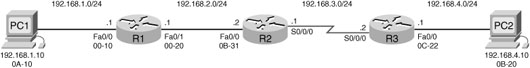
In the routing table shown in Example 18-1, the AD value is the first value listed in the brackets. You can see that the AD value for RIP routes is 120. You can also verify the AD value with the show ip protocols command as demonstrated in Example 18-2.

Table 18-2 shows a chart of the different administrative distance values for various routing protocols.

IGP Comparison Summary

Table 18-3 compares several features of the currently most popular IGPs: RIPv2, OSPF, and EIGRP.

Routing Loop Prevention

Without preventive measures, distance vector routing protocols could cause severe routing loops in the network. A routing loop is a condition in which a packet is continuously transmitted within a series of routers without ever reaching its intended destination network. A routing loop can occur when two or more routers have inaccurate routing information to a destination network.

A number of mechanisms are available to eliminate routing loops, primarily with distance vector routing protocols. These mechanisms include the following:

  Defining a maximum metric to prevent count to infinity: To eventually stop the incrementing of a metric during a routing loop, “infinity” is defined by setting a maximum metric value. For example, RIP defines infinity as 16 hops—an“unreachable” metric. When the routers “count to infinity,” they mark the route as unreachable.

  Hold-down timers: Used to instruct routers to hold any changes that might affect routes for a specified period of time. If a route is identified as down or possibly down, any other information for that route containing the same status, or worse, is ignored for a predetermined amount of time (the hold-down period) so that the network has time to converge.

  Split horizon: Used to prevent a routing loop by not allowing advertisements to be sent back through the interface they originated from. The split horizon rule stops a router from incrementing a metric and then sending the route back to its source.

  Route poisoning or poison reverse: Used to mark the route as unreachable in a routing update that is sent to other routers. Unreachable is interpreted as a metric that is set to the maximum.

  Triggered updates: A routing table update that is sent immediately in response to a routing change. Triggered updates do not wait for update timers to expire. The detecting router immediately sends an update message to adjacent routers.

  TTL Field in the IP Header: The purpose of the Time to Live (TTL) field is to avoid a situation in which an undeliverable packet keeps circulating on the network endlessly. With TTL, the 8-bit field is set with a value by the source device of the packet. The TTL is decreased by 1 by every router on the route to its destination. If the TTL field reaches 0 before the packet arrives at its destination, the packet is discarded and the router sends an ICMP error message back to the source of the IP packet.

Link-State Routing Protocol Features

Like distance vector protocols that send routing updates to their neighbors, link-state protocols send link-state updates to neighboring routers, which in turn forward that information to their neighbors, and so on. At the end of the process, like distance vector protocols, routers that use link-state protocols add the best routes to their routing tables, based on metrics. However, beyond this level of explanation, these two types of routing protocol algorithms have little in common.

Building the LSDB

Link-state routers flood detailed information about the internetwork to all the other routers so that every router has the same information about the internetwork. Routers use this link-state database (LSDB) to calculate the currently best routes to each subnet.

OSPF, the most popular link-state IP routing protocol, advertises information in routing update messages of various types, with the updates containing information called link-state advertisements (LSAs).

Figure 18-3 shows the general idea of the flooding process, with R8 creating and flooding its router LSA. Note that Figure 18-3 shows only a subset of the information in R8’s router LSA.

Figure 18-3 shows the rather basic flooding process, with R8 sending the original LSA for itself, and the other routers flooding the LSA by forwarding it until every router has a copy.

After the LSA has been flooded, even if the LSAs do not change, link-state protocols do require periodic reflooding of the LSAs by default every 30 minutes. However, if an LSA changes, the router immediately floods the changed LSA. For example, if Router R8’s LAN interface failed, R8 would need to reflood the R8 LSA, stating that the interface is now down.

Calculating the Dijkstra Algorithm

The flooding process alone does not cause a router to learn what routes to add to the IP routing table. Link-state protocols must then find and add routes to the IP routing table using the Dijkstra Shortest Path First (SPF) algorithm.

The SPF algorithm is run on the LSDB to create the SPF tree. The LSDB holds all the information about all the possible routers and links. Each router must view itself as the starting point, and each subnet as the destination, and use the SPF algorithm to build its own SPF tree to pick the best route to each subnet.

Figure 18-4 shows a graphical view of the results of the SPF algorithm run by router R1 when trying to find the best route to reach subnet 172.16.3.0/24 (based on Figure 18-3).

To pick the best route, a router’s SPF algorithm adds the cost associated with each link between itself and the destination subnet, over each possible route. Figure 18-4 shows the costs associated with each route beside the links, with the dashed lines showing the three routes R1 finds between itself and subnet X (172.16.3.0/24).

Table 18-4 lists the three routes shown in Figure 18-4, with their cumulative costs, showing that R1’s best route to 172.16.3.0/24 starts by going through R5.

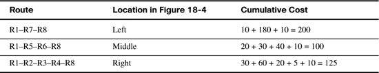
As a result of the SPF algorithm’s analysis of the LSDB, R1 adds a route to subnet 172.16.3.0/24 to its routing table, with the next-hop router of R5.

Convergence with Link-State Protocols

Remember, when an LSA changes, link-state protocols react swiftly, converging the network and using the currently best routes as quickly as possible. For example, imagine that the link between R5 and R6 fails in the internetwork of Figures 18-3 and 18-4. The following list explains the process R1 uses to switch to a different route.

1. R5 and R6 flood LSAs that state that their interfaces are now in a “down” state.

2. All routers run the SPF algorithm again to see if any routes have changed.

3. All routers replace routes, as needed, based on the results of SPF. For example, R1 changes its route for subnet X (172.16.3.0/24) to use R2 as the next-hop router.

These steps allow the link-state routing protocol to converge quickly—much more quickly than distance vector routing protocols.