
Stability
Keywords
Internal stability; Lyapunov stability; Input-output stability
There have been a large number of references on stability theory for ordinary differential equations, to mention a few [70, 76–86]. On the basis of the above references, this chapter serves a tutorial summary on stability of linear system, which covers the topics of internal stability, Lyapunov stability, and input-output stability.
5.1 Internal stability
Internal stability deals with boundedness properties and asymptotic behavior (as ![]() ) of solutions of the zero-input linear state equation
) of solutions of the zero-input linear state equation
While bounds on solutions might be of interest for fixed t0 and x0, or for various initial states at a fixed t0, we focus on boundedness properties that hole regardless of the choice of t0 or x0. In a similar fashion the concept we adopt relative to asymptotically zero solutions is independent of the choice of initial time. The reason is that these “uniform in t0” concepts are most appropriate in relation to input-output stability properties of linear state equations.
It is natural to begin by characterizing stability of linear state equation (5.1) in terms of bounds on the transition matrix Φ(t, π) for A(t). This leads to a well-known eigenvalue condition when A(t) is constant, but does not provide a generally useful stability test for time-varying examples because of the difficulty of computing Φ(t, π).
The first stability notion involves boundedness of solutions of Eq. (5.1). Because solutions are linear in the initial state, it is convenient to express the bound as a linear function of the norm of the initial state.
Definition 5.1.1
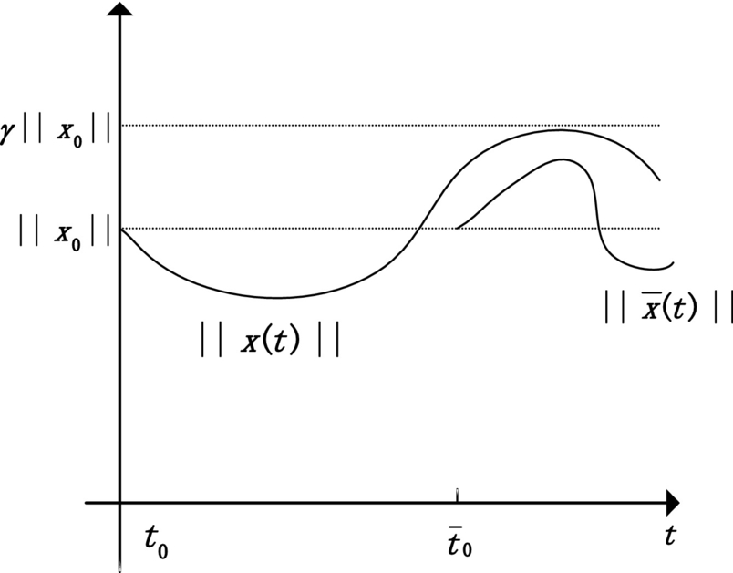
The linear state equation (5.1) is called uniformly stable if there exists a finite positive constant γ such that for any t0 and x0 the corresponding solution satisfies
Evaluation of Eq. (5.2) at t = t0 shows that the constant γ must satisfy γ ≥ 1. The adjective uniform in the definition refers precisely to the fact that γ must not depend on the choice of initial time, as illustrated in Fig. 5.1. A “nonuniform” stability concept can be defined by permitting γ to depend on the initial time, but this is not considered here except to show that there is a difference via a standard example.
Theorem 5.1.1
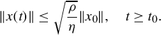
The linear state equation (5.1) is uniformly stable if and only if there exists a finite positive constant γ such that
for all t, τ such that t ≥ τ.
Proof
First suppose that such a γ exists. Then for any t0 and x0 the solution of Eq. (5.1) satisfies
and uniform stability is established.
For the reverse implication suppose that the state equation (5.1) is uniformly stable. Then there is a finite γ such that, for any t0 and x0, solutions satisfy
Given any t0 and ta ≥ t0, let xa be such that
(Such an xa exists by definition of the induced norm.) Then the initial state x(t0) = xa yields a solution of Eq. (5.1) that at time ta satisfies
Since ∥xa∥ = 1, this shows that ∥Φ(ta, t0)∥≤ γ. Because such an xa can be selected for any t0 and ta ≥ t0, the proof is complete.
5.1.1 Uniform exponential stability
Next we consider a stability property for Eq. (5.1) that addresses both boundedness and asymptotic behavior of solution. It implies uniform stability, and imposes an additional requirement that all solutions approach zero exponentially as ![]() .
.
Definition 5.1.2
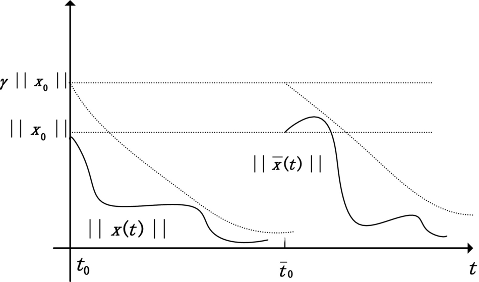
The linear state equation (5.1) is called uniformly exponentially stable if there exist finite positive constants γ, λ such that for any t0 and x0 the corresponding solution satisfies
Again γ is no less than unity, and the adjective uniform refers to the fact that γ and λ are independent of t0. This is illustrated in Fig. 5.2. The property of uniform exponential stability can be expressed in terms of an exponential bound on the transition matrix. The proof is similar to that of Theorem 5.1.1.
Theorem 5.1.2
The linear state equation (5.1) is uniformly exponentially stable if and only if there exist finite positive constants γ and λ such that
for all t, τ such that t ≥ τ.
Uniform stability and uniform exponential stability are the only internal stability concepts used in the sequel. Uniform exponential stability is the most important of the two, and another theoretical characterization of uniform exponentially stability for the bounded-coefficient case will prove useful.
Theorem 5.1.3
Suppose there exists a finite positive constant α such ∥A(t)∥≤ α for all t. Then the linear state equation (5.1) is uniformly exponentially stable if and only if there exists a finite positive constant β such that
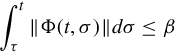
for all t, τ such that t ≥ τ.
Proof
If the state equation is uniformly exponentially stable, then by Theorem 5.1.1 there exist finite γ, λ > 0 such that
for all t, σ such that t ≥ σ. Then
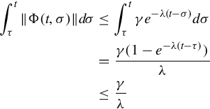
for all t, τ such that t ≥ τ. Thus Eq. (5.7) is established with ![]() .
.
Conversely suppose Eq. (5.7) holds. Basic calculus permit the representation
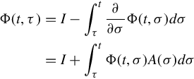
and thus
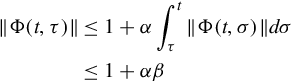
for all t, τ such that t ≥ τ. In completing this proof the composition property of the transition matrix is crucial. So long as t ≥ τ we can write, cleverly,
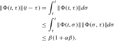
Therefore letting T = 2β(1 + αβ) and t = τ + T gives
for all τ. Applying Eqs. (5.8), (5.9), the following inequalities on time intervals of the form [τ + κT, τ + (κ + 1)T), where τ is arbitrary, are transparent:

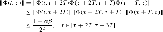
Continuing in this fashion shows that for any value of τ
Finally, choose ![]() and γ = 2(1 + αβ). Fig. 5.3 presents a plot of the corresponding decaying exponential and the bound (5.10), from which it is clear that
and γ = 2(1 + αβ). Fig. 5.3 presents a plot of the corresponding decaying exponential and the bound (5.10), from which it is clear that
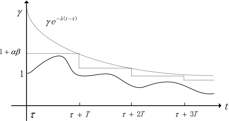
for all t, τ such that t ≥ τ. Uniform exponential stability thus is a consequence of Theorem 5.1.1.
An alternate form for the uniform exponential stability condition in Theorem 5.1.3 is

for all t. For time-invariant linear state equations, where Φ(t, σ) = eA(t−σ), an integration-variable change, in either form of the condition, shows that uniform exponential stability is equivalent to finiteness of
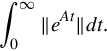
The adjective “uniform” is superfluous in the time-invariant case, and we will drop it in clear contexts. Though exponential stability usually is called asymptotic stability when discussing time-invariant linear state equations, we retain the term exponential stability.
Combining an explicit representation for eAt with the finiteness condition on Eq. (5.11) yields a better-known characterization of exponential stability.
Proof
Suppose the eigenvalue condition holds. Then writing eAt in the explicit form, where λ1, ……, λm are the distinct eigenvalues of A, gives

Since ![]() , the bound shows that the right side is finite, and exponential stability follows.
, the bound shows that the right side is finite, and exponential stability follows.
If the negative-real-part eigenvalue condition on A fails, then appropriate selection of an eigenvalue of A as an initial state can be used to show that the linear state equation is not exponentially stable. Suppose first that a real eigenvalue λ is nonnegative, and let p be an associated eigenvector. Then the power series representation for the matrix exponential easily shows that
For the initial state x0 = p, it is clear that the corresponding solution of Eq. (5.1), x(t) = eλtp, does not go to zero as ![]() . Thus the state equation is not exponentially stable.
. Thus the state equation is not exponentially stable.
Now suppose that λ = σ + iω is a complex eigenvalue of A with σ > 0. Again let p be an eigenvector associate with λ, written
Then
and thus
does not approach zero as ![]() . Therefore at least one of the real initial states x0 = Re[p] or x0 = Im[p] yields a solution that does not approach zero as
. Therefore at least one of the real initial states x0 = Re[p] or x0 = Im[p] yields a solution that does not approach zero as ![]() .
.
This proof, with a bit of elaboration, shows also that ![]() is a necessary and sufficient condition for uniform exponential stability in the time-invariant case. The corresponding statement is not true for time-invariant linear state equations.
is a necessary and sufficient condition for uniform exponential stability in the time-invariant case. The corresponding statement is not true for time-invariant linear state equations.
5.1.2 Uniform asymptotic stability
Definition 5.1.3
The linear state equation (5.1) is called uniformly asymptotically stable if it is uniformly stable, and if given any positive constant δ there exists a positive T such that for any t0 and x0 the corresponding solution satisfies
Note that the elapsed time T, until the solution satisfies the bound (5.13), must be independence of the initial time. Some of the same tools used in proving Theorem 5.1.3 can be used to show that this “elapsed-time uniformity” is the key to uniform exponential stability.
Proof
Suppose that the state equation is uniformly exponentially stable, that is, there exist finite, positive γ and λ such that ∥Φ(t, τ)∥≤ γe−λ(t−τ) whenever t ≥ τ. Then the state equation clearly is uniformly stable. To show it is uniformly asymptotically stable, for a given σ > 0 pick T such that ![]() . Then for any t0 and x0, and t ≥ t0 + T,
. Then for any t0 and x0, and t ≥ t0 + T,

This demonstrates uniform asymptotic stability.
Conversely suppose the state equation is uniformly asymptotically stable. Uniform stability is implied by definition, so there exists a positive γ such that
for all t, τ such that t ≥ τ. Select ![]() , and by Definition 5.1.3 let T be such that Eq. (5.13) is satisfied. Then given a t0, let xa be such that ∥xa∥ = 1, and
, and by Definition 5.1.3 let T be such that Eq. (5.13) is satisfied. Then given a t0, let xa be such that ∥xa∥ = 1, and
With the initial state x(t0) = xa, the solution of Eq. (5.1) satisfies

from which
Of course such an xa exists for any given t0, so the argument compels Eq. (5.15) for any t0. Now uniform exponential stability is implied by Eqs. (5.14), (5.15), exactly as in the proof of Theorem 5.1.3.
5.1.3 Lyapunov transformation
The stability concepts under discussion are properties of particular linear state equation that presumably represent a system of interest in terms of physically meaningful variables. A basic question involves preservation of stability properties under a state variable change. Since time-varying variable changes are permitted, simple scalar examples can be generated to show that, for example, uniform stability can be created or destroyed by variable change. To circumvent this difficulty we must limit attention to a particular class of state variable changes.
Definition 5.1.4
An n × n matrix P(t) that is continuously differentiable and invertible at each t is called a Lyapunov transformation if there exist finite positive constants ρ and η such that for all t
A condition equivalent to Eq. (5.16) is existence of a finite positive constant ρ such that for all t
The lower bound on |detP(t)| implies an upper bound on ∥P−1(t)∥.
Reflecting on the effect of a state variable change on the transition matrix, a detailed proof that Lyapunov transformations preserve stability properties is perhaps belaboring the evident.
Theorem 5.1.6
Suppose the n × n matrix P(t) is Lyapunov transformation. Then the linear state equation (5.1) is uniformly stable (respectively, uniformly exponentially stable) if and only if the state equation
is uniformly stable (respectively, uniformly exponentially stable).
Proof
The linear state equations (5.1) and (5.17) are related by the variable change z(t) = P−1(t)x(t), and we note that the properties required of a Lyapunov transformation subsume those required of a variable change. Thus the relation between the two transition matrices is
Now suppose Eq. (5.1) is uniformly stable. Then there exists γ such that ∥Φx(t, τ)∥≤ γ for all t, τ such that t ≥ τ, and, from Eq. (5.16)

for all t, τ such that t ≥ τ. This shows that Eq. (5.17) is uniformly stable. An obviously similar argument applied to
shows that if Eq. (5.17) is uniformly stable, then Eq. (5.1) is uniformly stable. The corresponding demonstrations for uniform exponential stability are similar.
The Floquet decomposition for T-periodic state equations provides a general illustration. Since P(t) is the product of a transition matrix and a matrix exponential, it is continuously differentiable with respect to t. Since P(t) is invertible, by continuity arguments there exist ρ, η > 0 such that Eq. (5.16) holds for all t in any P(t) is Lyapunov transformation. It is easy to verify that z(t) = P−1(t)x(t) yields the time-invariant linear state equation
By this connection stability properties of the original T-periodic state equation are equivalent to stability properties of a time-invariant linear state equation (though, it must be noted, the time-invariant state equation in general is complex).
5.2 Lyapunov stability
The origin of Lyapunov’s so-called direct method for stability assessment is the notion that total energy of an unforced, dissipative mechanical system decreases as the state of the system evolves in time. Therefore the state vector approaches a constant value corresponding to zero energy as time increases. Phrased more generally, stability properties involve the growth properties of solutions of the state equation, and these properties can be measured by suitable (energy-like) scalar function of the state vector. The problem is finding a suitable scalar function.
5.2.1 Introduction
To illustrate the basic idea we consider conditions that imply all solutions of the linear state equation
are such that ∥x(t)∥2 monotonically decreases as ![]() . For any solution x(t) of Eq. (5.19), the derivative of the scalar function
. For any solution x(t) of Eq. (5.19), the derivative of the scalar function
with respect to t can be written as

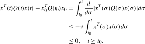
In this computation ![]() is replaced by A(t)x(t) precisely because x(t) is a solution of Eq. (5.19). Suppose that the quadratic form on the right side of Eq. (5.21) is negative definite, that is, suppose the matrix AT(t) + A(t) is negative definite at each t. Then, as shown in Fig. 5.4, ∥x(t)∥2 decreases as t increases. Further we can show that if this negative definiteness does not asymptotically vanish, that is, if there is a constant ν > 0 such that AT(t) + A(t) ≤−νI for all t, then ∥x(t)∥2 goes to zero as
is replaced by A(t)x(t) precisely because x(t) is a solution of Eq. (5.19). Suppose that the quadratic form on the right side of Eq. (5.21) is negative definite, that is, suppose the matrix AT(t) + A(t) is negative definite at each t. Then, as shown in Fig. 5.4, ∥x(t)∥2 decreases as t increases. Further we can show that if this negative definiteness does not asymptotically vanish, that is, if there is a constant ν > 0 such that AT(t) + A(t) ≤−νI for all t, then ∥x(t)∥2 goes to zero as ![]() . Notice that the transition matrix for A(t) is not needed in this calculation, and growth properties of the scalar function (5.20) depend on sign-definiteness properties of the quadratic form in Eq. (5.21). Admittedly this calculation results in a restrictive sufficient condition—negative definiteness of AT(t) + A(t)—for a type of asymptotic stability. However, more general scalar functions than Eq. (5.20) can be considered.
. Notice that the transition matrix for A(t) is not needed in this calculation, and growth properties of the scalar function (5.20) depend on sign-definiteness properties of the quadratic form in Eq. (5.21). Admittedly this calculation results in a restrictive sufficient condition—negative definiteness of AT(t) + A(t)—for a type of asymptotic stability. However, more general scalar functions than Eq. (5.20) can be considered.

Formalization of the above discussion involves somewhat intricate definitions of time-dependent quadratic forms that are useful as scalar functions of the state vector of Eq. (5.19) for stability purpose. Such quadratic forms are called quadratic Lyapunov functions. They can be written as xTQ(t)x, where Q(t) is assumed to be symmetric and continuously differentiable for all t. If x(t) is any solution of Eq. (5.19) for t ≥ t0, then we are interested in the behavior of the real quantity xT(t)Q(t)x(t) for t ≥ t0. This behavior can be assessed by computing the time derivative using the product rule, and replacing ![]() by A(t)x(t) to obtain
by A(t)x(t) to obtain
To analyze stability properties, various bounds are required on quadratic Lyapunov functions and on the quadratic forms (5.22) that arise as their derivatives along solutions of Eq. (5.19). These bounds can be expressed in alternative ways. For example, the condition that there exists a positive constant η such that
for all t is equivalent by definition to existence of a positive η such that
for all t and all n × 1 vectors x. Yet another way to write this is to require the existence of a symmetric, positive-definite constant matrix M such that
for all t and all n × 1 vectors x. The choice is largely a matter of taste, and the most economical form is adopted here.
5.2.2 Uniform stability
We begin with a sufficient condition for uniform stability. The presentation style throughout is to list the requirement on Q(t) so that the corresponding quadratic form can be used to prove the desired stability property.
Theorem 5.2.1
The linear state equation (5.19) is uniformly stable if there exists an n × n matrix Q(t) that for all t is symmetric, continuously differentiable, and such that
where η and ρ are finite positive constants.
Proof
Given any t0 and x0, the corresponding solution x(t) of Eq. (5.19) is such that, from Eqs. (5.22), (5.24),

Using the inequalities in Eq. (5.23) we obtain
and then
Therefore
Since Eq. (5.25) holds for any x0 and t0, the state equation (5.19) is uniformly stable by definition.
Typically it is profitable to use a quadratic Lyapunov function to obtain stability conditions for linear state equations, rather than a particular instance.
5.2.3 Uniform exponential stability
Theorem 5.2.2
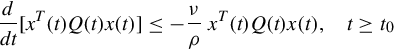
The linear state equation (5.19) is uniformly exponentially stable if there exists an n × n matrix function Q(t) that for all t is symmetric, continuously differentiable, and such that
when η, ρ, and ν are finite positive constants.
Proof
For any t0, x0, and corresponding solution x(t) of the state equation, the inequality (5.27) gives
Also from Eq. (5.26)

Therefore
and this implies, after multiplication by the appropriate exponential integrating factor, and integrating from t0 to t,
Summoning Eq. (5.26) again,

which in turn gives
Noting that Eq. (5.29) holds for any x0 and t0, and taking the positive square root of both sides, uniform exponential stability is established.
For n = 2 and constant Q(t) = Q, Theorem 5.22 admits a simple pictorial representation. The condition (5.26) implies that Q is positive definite, and therefore the level curves of the real-valued function xTQx are ellipses in the (x1, x2)-plane. The condition (5.27) implies that for any solution x(t) of the state equation the value of xT(t)Qx(t) is decreasing as t increases. Thus a plot of the solution x(t) on the (x1, x2)-plane crosses smaller-value level curves as t increases, as shown in Fig. 5.5. Under the same assumptions, a similar pictorial interpretation can be given for Theorem 5.2.1. Note that if Q(t) is not constant, the level curves vary with t and the picture is much less informative.

Just in case it appears that stability of linear state equations is reasonably intuitive. A first guess is that the state equation is uniformly exponentially stable if a(t) is continuous and positive for all t, though suspicions might arise if ![]() as
as ![]() . These suspicious would be well founded, but what is more surprising is that there are other obstructions to uniform exponential stability.
. These suspicious would be well founded, but what is more surprising is that there are other obstructions to uniform exponential stability.
The stability criteria provided by the preceding theorems are sufficient conditions that depend on skill in selecting an appropriate Q(t). It is comforting to show that there indeed exists a suitable Q(t) for a large class of uniformly exponentially stable linear state equations. The dark side is that it can be roughly as hard to compute Q(t) as it is to compute the transition matrix for A(t).
Theorem 5.2.3
Suppose that the linear state equation (5.19) is uniformly exponentially stable, and there exists a finite constant α such that ∥A(t)∥≤ α for all t. Then

satisfies all the hypotheses of Theorem 5.2.2.
Proof
First we show that the integral converges for each t, so that Q(t) is well defined. Since the state equation is uniformly exponentially stable, there exists positive γ and λ such that
for all t, t0 such that t ≥ t0. Thus

for all t. This calculation also defines ρ in Eq. (5.26). Since Q(t) clearly is symmetric and continuously differentiable at each t, it remains only to show that there exist η, ν > 0 as needed in Eqs. (5.26), (5.27). To obtain ν, differentiation of Eq. (5.30) gives
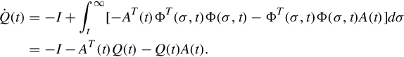
That is
and clearly a valid choice for ν in Eq. (5.27) is ν = 1. Finally it must be shown that there exists a positive η such that Q(t) ≥ ηI for all t, and for this we set up an adroit maneuver. For any x and t
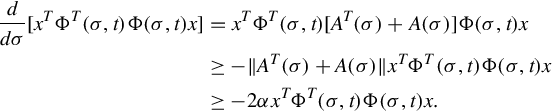
Using the fact that Φ(σ, t) approaches zero exponentially as ![]() , we integrate both sides to obtain
, we integrate both sides to obtain

Evaluating the integral gives
or
for all t. Thus with the choice ![]() all hypotheses of Theorem 5.2.2 are satisfied.
all hypotheses of Theorem 5.2.2 are satisfied.
5.2.4 Instability
Quadratic Lyapunov function also can be used to develop instability criteria of various types. One example is the following result that, except for one value of t, does not involve a sign-definiteness assumption on Q(t).
Theorem 5.2.4
Suppose there exists an n × n matrix function Q(t) that for all t is symmetric, continuously differentiable, and such that
where ρ and ν are finite positive constants. Also suppose there exists a ta such that Q(ta) is not positive semidefinite. Then the linear state equation (5.19) is not uniformly stable.
Proof
Suppose x(t) is the solution of Eq. (5.19) with t0 = ta and x0 = xa such that ![]() . Then, from Eq. (5.34),
. Then, from Eq. (5.34),
One consequence of this inequality, Eq. (5.33), and the choice of x0 and t0, is
and a further consequence is that
Using Eqs. (5.33), (5.36) gives

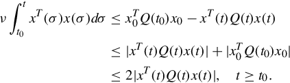
The state equation can be shown to be not uniformly stable by proving that x(t) is unbounded. This we do by a contradiction argument. Suppose that there exists a finite γ such that ∥x(t)∥≤ γ, for all t ≥ t0. Then Eq. (5.37) gives
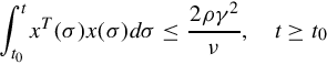
and the integrand, which is a continuously differentiable scalar function, must go to zero as ![]() . Therefore x(t) must also go to zero, and this implies that Eq. (5.35) is violated for sufficiently large t. The contradiction proves that x(t) cannot be a bounded solution.
. Therefore x(t) must also go to zero, and this implies that Eq. (5.35) is violated for sufficiently large t. The contradiction proves that x(t) cannot be a bounded solution.
5.2.5 Time-invariant case
In the time-invariant case quadratic Lyapunov function with constant Q can be used to connect Theorem 5.2.2 with the familiar eigenvalue condition for exponential stability. If Q is symmetric and positive definite, then Eq. (5.26) is satisfied automatically. However, rather than specifying such a Q and checking to see if a positive ν exists such that Eq. (5.27) is satisfied, the approach can be reversed. Choose a positive definite matrix M, for example M = νI, where ν > 0. If there exists a symmetric, positive-definite Q such that
then all the hypotheses of Theorem 5.2.2 are satisfied. Therefore the associated linear state equation
is exponentially stable, all eigenvalues of A have negative real parts. Conversely the eigenvalues of A enter the existence question for solution of the Lyapunov equation (5.38).
Theorem 5.2.5
Given an n × n matrix A, if M and Q are symmetric, positive-definite, n × n matrices satisfying Eq. (5.38), then all eigenvalues of A have negative real parts. Conversely if all eigenvalues of A have negative real parts, then for each symmetric n × n matrix M there exists a unique solution of Eq. (5.38) given by
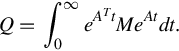
Furthermore, if M is positive definite, then Q is positive definite.
Proof
For the converse, if all eigenvalues of A have negative real parts, it is obvious that the integral in Eq. (5.39) converges, so Q is well defined. To show that Q is a solution of Eq. (5.38), we calculate

To prove this solution is unique, suppose Qa also is a solution. Then
But this implies
from which
Integrating both sides from 0 to ![]() gives
gives
That is, Qa = Q. Now suppose that M is positive definite. Clearly Q is symmetric. To show it is positive definite simply note that for a zero n × 1 vector x
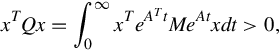
since the integrand is a positive scalar function. (In detail, eAtx≠0 for t ≥ 0, so positive definiteness of M shows that the integrand is positive for all t ≥ 0.)
5.3 Input-output stability
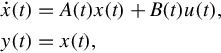
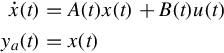
In this section we address stability properties appropriate to the input-output behavior (zero-state response) of the linear state equation

That is, the initial state is set to zero, and attention is focused on the boundedness of the response to bounded inputs. There is no D(t)u(t) term in Eq. (5.42) because a bounded D(t) does not affect the treatment, while an unbounded D(t) provides an unbounded response to an appropriate constant input. Of course the input-output behavior of Eq. (5.42) is specified by the impulse response
and stability results are characterized in terms of boundedness properties of ∥G(t, σ)∥. (Notice in particular that the weighting pattern is not employed.) For the time-invariant case, input-output stability also is characterized in terms of the transfer function of the linear state equation.
5.3.1 Uniform bounded-input bounded-output stability
Bounded-input, bounded-output stability is most simply discussed in terms of the largest value (over time) of the norm of the input signal, ∥u(t)∥, in comparison to the largest value of the corresponding response norm ∥y(t)∥. More precisely we use the standard notion of supremum. For example,
is defined as the smallest constant such that u(t) ≤ ν for t ≥ t0. If no such bound exists, we write
The basic notion is that the zero-state response should exhibit finite “gain” in terms of the input and output suprema.
Definition 5.3.1
The linear state equation (5.42) is called uniformly bounded-input, bounded-output stable if there exists a finite constant η such that for any t0 and any input signal u(t) the corresponding zero-state response satisfies
The adjective “uniform” does double duty in this definition. It emphasizes the fact that the same η works for all values of t0, and that the same η works for all input signals. An equivalent definition based on the pointwise norms of u(t) and y(t) is explored.
Theorem 5.3.1
The linear state equation (5.42) is uniformly bounded-input, bounded-output stable if and only if there exists a finite constant ρ such that for all t, τ with t ≥ τ,

Proof
Assume first that such a ρ exists. Then for any t0 and any input defined for t ≥ t0, the corresponding zero-state response of Eq. (5.42) satisfies
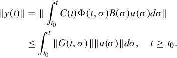
Replacing ∥u(σ)∥ by its supremum over σ ≥ t0, and using Eq. (5.45),
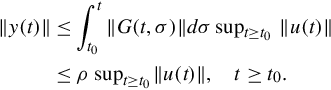
Therefore, taking the supremum of the left side over t ≥ t0, Eq. (5.44) holds with η = ρ, and the state equation is uniformly bounded-input, bounded-output stable.
Suppose now that Eq. (5.42) is uniformly bounded-input, bounded-output stable. Then there exists a constant η so that, in particular, the zero-state response for any t0 and any input signal such that
satisfies
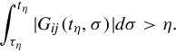
To set up a contradiction argument, suppose no finite ρ exists that satisfies Eq. (5.45). In other words for any given constant ρ there exist τρ and tρ > τρ such that

Taking ρ = η, that there exist τη, tη > τη, and indices i, j such that the i, j-entry of the impulse response satisfies
With t0 = τη consider the m × 1 input signal u(t) defined for t ≥ t0 as follows. Set u(t) = 0 for t > tη, and for t ∈ [t0, tη] set every component of u(t) to zero except for the jth-component given by (the piecewise-continuous signal)

This input signal satisfies ∥u(t)∥≤ 1, for all t ≥ t0, but the ith-component of the corresponding zero-state response satisfies, by Eq. (5.46),
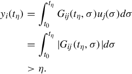
Since ∥y(tη)∥≥∥yi(tη)∥, a contradiction is obtained that completes the proof.
An alternate expression for the condition in Theorem 5.3.1 is that there exist a finite ρ such that for all t

For a time-invariant linear state equation, G(t, σ) = G(t, −σ), and the impulse response customarily is written as G(t) = CeAtB, t ≥ 0. Then a change of integration variable shows that a necessary and sufficient condition for uniform bounded-input, bounded-output stability for a time-invariant state equation is finiteness of the integral

5.3.2 Relation to uniform exponential stability
We now turn to establishing connections between uniform bounded-input, bounded-output stability and the property of uniform exponential stability of the zero-input response.
Lemma 5.3.1
Suppose the linear state equation (5.42) is uniformly exponentially stable, and there exist finite constant β and μ such that for all t
Then the state equation also is uniformly bounded-input, bounded-output stable.
Proof
Using the transition matrix bound implied by uniform exponential stability,

for all t, τ with t ≥ τ. Therefore the state equation is uniformly bounded-input, bounded-output stable by Theorem 5.3.1.
That coefficient bounds as in Eq. (5.48) are needed to obtain the implication in Lemma 5.3.1 should be clear. However, the simple proof might suggest that uniform exponential stability is a needlessly strong condition for uniform bounded-input, bounded-output stability.
In developing implication of uniform bounded-input, bounded-output stability for uniform exponential stability, we need to strengthen the usual controllability and observability properties. Specifically it will be assumed that these properties are uniform in time in special way. For simplicity, admittedly a commodity in short supply for the next few pages, the development is subdivided into two parts. First we deal with linear state equations where the output is precisely the state vector (C(t) is the n × n identity). In this instance the natural terminology is uniform bounded-input, bounded-state stability.
Theorem 5.3.2
Suppose for the linear state equation
there exist finite positive constants α, β, ε, and δ such that for all t
Then the state equation is uniformly bounded-input, bounded-state stable if and only if it is uniformly exponentially stable.
Proof
One direction of proof is supplied by Lemma 5.3.1, so assume the linear state equation (5.42) is uniformly bounded-input, bounded-state stable. Applying Theorem 5.3.1 with C(t) = I, there exists a finite constant ρ such that

for all t, τ such that t ≥ τ. We next show that this implies existence of a finite constant ψ such that

for all t, τ such that t ≥ τ, and thus conclude uniform exponential stability.
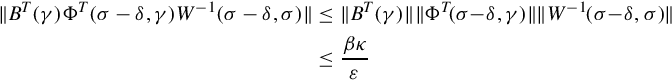
First, since A(t) is bounded, corresponding to the constant δ in Eq. (5.49) there exist a finite constant κ such that
Second, the lower bound on the controllability Gramian in Eq. (5.49) gives
for all t, and therefore
for all t. In particular these bounds show that
for all σ, γ satisfying |σ − δ − γ|≤ δ. Therefore writing
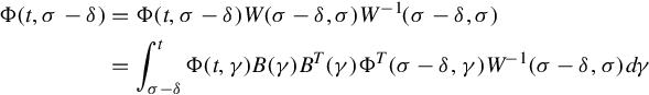
we obtain, since σ − δ ≤ γ ≤ σ implies |σ − δ − γ|≤ δ,
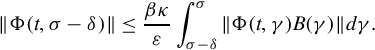
Then

The proof can be completed by showing that the right side of Eq. (5.45) is bounded for all t, τ such that t ≥ τ.
In the inside integral on the right side of Eq. (5.45), change the integration variable from γ to ξ = γ − σ + δ, and then interchange the order of integration to write the right side of Eq. (5.45) as

In the inside integral in this expression, change the integration variable from σ − δ to ζ = ξ + σ − δ to obtain

Since 0 ≤ ξ ≤ δ we can use Eqs. (5.50), (5.51) with the composition property to bound the inside integral in Eq. (5.53)) as

Therefore Eq. (5.52) becomes

This holds for all t, τ such that t ≥ τ, so uniform exponential stability of linear state equation with C(t) = I.
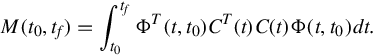
To address the general case, where C(t) is not an identity matrix, recall that the observability Gramian for the state equation (5.42) is defined by
Theorem 5.3.3
Suppose that for the linear state equation (5.42) there exist finite positive constants α, β, μ, ε1, δ1, ε2, and δ2 such that
for all t. Then the state equation is uniformly bounded-input, bounded-output stable if and only if it is uniformly exponentially stable.
Proof
Again uniform exponential stability implies uniform bounded-input, bounded-output stability by Lemma 5.3.1. So suppose that Eq. (5.42) is uniformly bounded-input, bounded-output stable, and η is such that the zero-state response satisfies
for all inputs u(t). We will show that the associated state equation with C(t) = I, namely,
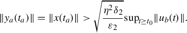
also is uniformly bounded-input, bounded-state stable. To set up a contradiction argument, assume the negation. Then for the positive constant ![]() there exists a t0, ta > t0, and bounded input signal ub(t) such that
there exists a t0, ta > t0, and bounded input signal ub(t) such that
Furthermore we can assume that ub(t) satisfies ub(t) = 0 for t > ta. Applying this input to Eq. (5.42), keeping the same initial time t0, the zero-state response satisfies

Invoking the hypothesis on the observability Gramian, and then Eq. (5.58),
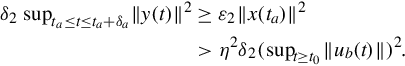
Using elementary properties of the supremum, including
yields
Thus we have shown that the bounded input ub(t) is such that bound (5.56) for uniform bounded-input, bounded-output stability of Eq. (5.42) is violated. This contradiction implies Eq. (5.57) is uniformly bounded-input, bounded-state stable. Then by Theorem 5.3.2 the state equation (5.57) is uniformly exponentially stable and, hence, Eq. (5.42) also is uniformly exponentially stable.
5.3.3 Time-invariant case
Complicated and seemingly contrived manipulations in the proofs of Theorems 5.3.2 and 5.3.3 motivate separate consideration of the time-invariant case. In the time-invariant setting, simpler characterizations of stability properties, and of controllability and observability, yield more straightforward proofs. For the linear state equation
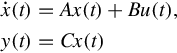
the main task in proving an analog of Theorem 5.3.3 is to show that controllability, observability, and finiteness of

imply finiteness of

Proof
Clearly exponential stability implies uniform bounded-input, bounded-output stability since

Conversely, suppose Eq. (5.43) is uniformly bounded-input, bounded-output stable. Then Eq. (5.61) is finite, and this implies
Using a representation for the matrix exponential, we can write the impulse response in the form

where λ1, …, λl are the distinct eigenvalues of A, and the Gkj are p × m constant matrices. Then

If we suppose that this function does not go to zero, then from a comparison with Eq. (5.63) we arrive at a contradiction with Eq. (5.62). Therefore
That is,
This reasoning can be repeated to show that any time derivative of the impulse response goes to zero as ![]() . Explicitly,
. Explicitly,
These data implies

Using the controllability and observability hypotheses, select n linearly independent columns of the controllability matrix to form an invertible matrix Wa, and n linearly independent rows of the observability matrix to form an invertible Ma. Then, from Eq. (5.64),
Therefore
For some purposes it is useful to express the condition for uniform bounded-input, bounded-output stability of Eq. (5.60) in terms of the transfer function G(s) = C(sI−A)−1B. We use the familiar terminology that a pole of G(s) is a (complex, in general) value of s, say s0, such that for some i, j, ![]()
If each entry of G(s) has negative-real-part poles, then a partial-fraction-expansion computation shows that each entry of G(t) has a “sum of t-multiplied exponentials” form, with negative-real-part exponents. Therefore

is finite, and any realization of G(s) is uniformly bounded-input, bounded-output stable. On the other hand if Eq. (5.65) is finite, then the exponential terms in any entry of G(t) must have negative real parts. (Write a general entry in terms of distinct exponentials, and use a contradiction argument.) But then every entry of G(s) has negative-real-part poles.
Supplying this reasoning with a little more specificity proves a standard result.
For the time-invariant linear state equation (5.60), the relation between input-output stability and internal stability depends on whether all distinct eigenvalues of A appear as poles of G(s) = C(sI−A)−1B. Controllability and observability guarantee that this is the case. (Unfortunately, eigenvalues of A sometimes are called “poles of A,” a loose terminology that at best obscures delicate distinctions.)