
Nonstandard H∞ control problem
A generalized chain-scattering representation approach
Abstract
The nonstandard ![]() control problem is the case where the direct feedthroughs from the input to the error and from the exogenous signal to the output are not necessarily of full rank. This problem is reformulated based on the generalized chain-scattering representation (GCSR). The GCSR approach leads naturally to a generalization of the homographic transformation. The state-space realization for this generalized homographic transformation and a number of fundamental cascade structures of the
control problem is the case where the direct feedthroughs from the input to the error and from the exogenous signal to the output are not necessarily of full rank. This problem is reformulated based on the generalized chain-scattering representation (GCSR). The GCSR approach leads naturally to a generalization of the homographic transformation. The state-space realization for this generalized homographic transformation and a number of fundamental cascade structures of the ![]() control systems are further studied in a unified framework of GCSR. Certain sufficient conditions for the solvability of the nonstandard
control systems are further studied in a unified framework of GCSR. Certain sufficient conditions for the solvability of the nonstandard ![]() control problem are therefore established via a ((J, J′))-lossless factorization of GCSR. These results present extensions to Kimura’s results on the chain-scattering representation (CSR) approach to the
control problem are therefore established via a ((J, J′))-lossless factorization of GCSR. These results present extensions to Kimura’s results on the chain-scattering representation (CSR) approach to the ![]() control in the standard case.
control in the standard case.
Keywords
![]() control systems; The generalized chain-scattering representation (GCSR); State-space realization; Nonstandard
control systems; The generalized chain-scattering representation (GCSR); State-space realization; Nonstandard ![]() control problem; ((J, J′))-lossless factorization; Chain-scattering representation (CSR)
control problem; ((J, J′))-lossless factorization; Chain-scattering representation (CSR)
The nonstandard ![]() control problem is the case where the direct feedthroughs from the input to the error and from the exogenous signal to the output are not necessarily of full rank. This problem is reformulated based on the generalized chain-scattering representation (GCSR). The GCSR approach leads naturally to a generalization of the homographic transformation. The state-space realization for this generalized homographic transformation and a number of fundamental cascade structures of the
control problem is the case where the direct feedthroughs from the input to the error and from the exogenous signal to the output are not necessarily of full rank. This problem is reformulated based on the generalized chain-scattering representation (GCSR). The GCSR approach leads naturally to a generalization of the homographic transformation. The state-space realization for this generalized homographic transformation and a number of fundamental cascade structures of the ![]() control systems are further studied in a unified framework of GCSR. Certain sufficient conditions for the solvability of the nonstandard
control systems are further studied in a unified framework of GCSR. Certain sufficient conditions for the solvability of the nonstandard ![]() control problem are therefore established via a (
control problem are therefore established via a (![]() )-lossless factorization of GCSR. These results present extensions to Kimura’s results on the chain-scattering representation (CSR) approach to the
)-lossless factorization of GCSR. These results present extensions to Kimura’s results on the chain-scattering representation (CSR) approach to the ![]() control in the standard case.
control in the standard case.
14.1 Introduction
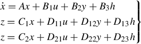
Consider the plant

where ![]() ,
, ![]() ,
, ![]() , and
, and ![]() are the controlled error, the observation output, the exogenous input, and the control input, respectively. The
are the controlled error, the observation output, the exogenous input, and the control input, respectively. The ![]() control problem is to find a controller given by
control problem is to find a controller given by
which internally stabilizes the closed-loop system and satisfies ![]() , where Φ is the closed-loop transfer function from w to z, which is generally called a linear fractional transformation in the control literature and is denoted [22] by LF(P;K), i.e.,
, where Φ is the closed-loop transfer function from w to z, which is generally called a linear fractional transformation in the control literature and is denoted [22] by LF(P;K), i.e.,
Concerning the above problem, one of the assumptions is the following
When the plant satisfies the above assumption, the ![]() control problem is called [37] the regular or standard case, while the case where the above assumption does not hold is referred [120] to a singular
control problem is called [37] the regular or standard case, while the case where the above assumption does not hold is referred [120] to a singular ![]() control problem. We do not make the above assumption, the considered problem is thus nonstandard, which includes both the regular case and the singular case. From a system point of view, since no measurement is error free and no control action is costless [117] it is physically reasonable and general (see, e.g., [90]) to assume that the dimension of z is at least that of u, while the dimension of w must be at least that of y, without loss of generality only the right noninvertibility of P21 is thus considered in the following development. It should also be noted that, in Assumption (A) rank P21 = q means that, rank P21(jω) = q, ∀ω ∈R and rank
control problem. We do not make the above assumption, the considered problem is thus nonstandard, which includes both the regular case and the singular case. From a system point of view, since no measurement is error free and no control action is costless [117] it is physically reasonable and general (see, e.g., [90]) to assume that the dimension of z is at least that of u, while the dimension of w must be at least that of y, without loss of generality only the right noninvertibility of P21 is thus considered in the following development. It should also be noted that, in Assumption (A) rank P21 = q means that, rank P21(jω) = q, ∀ω ∈R and rank ![]() .
.
Several approaches (e.g., [25, 36, 37, 121], and references therein) have already been proposed to solve the regular ![]() control problem both in the state-space framework and in the input-output operator-theoretic techniques. The singular
control problem both in the state-space framework and in the input-output operator-theoretic techniques. The singular ![]() control problem has attracted considerable research interests in the last few years [120, 122]. For a monograph on this subject, one can refer to [122–124] considered controller design for the singular
control problem has attracted considerable research interests in the last few years [120, 122]. For a monograph on this subject, one can refer to [122–124] considered controller design for the singular ![]() control problem based on the linear matrix inequality (LMI) approach. One basic observation to the aforementioned contributions on this theme is, however, that the problem is generally attacked in the state-space framework. Although state-space techniques are powerful for computing solutions, and are growing even more so with the advent of efficient numerical techniques, they do not always give physical insight into the nature of problems and bear fundamental limitations. Such insight can be obtained much more effectively using input-output techniques that allow solutions to be revealed and understood in their most transparent forms, and without the often obscuring one details that occur in specific problems.
control problem based on the linear matrix inequality (LMI) approach. One basic observation to the aforementioned contributions on this theme is, however, that the problem is generally attacked in the state-space framework. Although state-space techniques are powerful for computing solutions, and are growing even more so with the advent of efficient numerical techniques, they do not always give physical insight into the nature of problems and bear fundamental limitations. Such insight can be obtained much more effectively using input-output techniques that allow solutions to be revealed and understood in their most transparent forms, and without the often obscuring one details that occur in specific problems.
Recently Kimura [22, 90] has developed the CSR, and it was successfully used there to provide a unified framework of ![]() control theory. In this new framework, the
control theory. In this new framework, the ![]() control problem is essentially reduced to a J-lossless factorization of the CSR of the plant. The J-lossless conjugation then provides a powerful tool for computing the required factorization. Kimura’s CSR approach seems to be the most compact theory and the simplest method to the regular
control problem is essentially reduced to a J-lossless factorization of the CSR of the plant. The J-lossless conjugation then provides a powerful tool for computing the required factorization. Kimura’s CSR approach seems to be the most compact theory and the simplest method to the regular ![]() control problem. The known CSR approach is, however, not applicable to the singular
control problem. The known CSR approach is, however, not applicable to the singular ![]() control problem. This situation may improve with the advent of [125]. In [125] Kimura’s results on CSR has been extended to the general case in which the condition (A) is essentially relaxed. From an input-output consistency point of view, the GCSR emerges and is successfully used there to characterize the cascade structure property and the symmetry of general plants in a general setting.
control problem. This situation may improve with the advent of [125]. In [125] Kimura’s results on CSR has been extended to the general case in which the condition (A) is essentially relaxed. From an input-output consistency point of view, the GCSR emerges and is successfully used there to characterize the cascade structure property and the symmetry of general plants in a general setting.
The main motivation of our current work presented herein is to extend Kimura’s results [22, 90] on CSR approach to the ![]() control from the standard case to the nonstandard case by using the GCSR approach [125]. To this end, the nonstandard
control from the standard case to the nonstandard case by using the GCSR approach [125]. To this end, the nonstandard ![]() control problem is first reformulated based on the GCSR. The GCSR approach then leads naturally to a generalization of the homographic transformation. The state-space realization for this generalized homographic transformation and a number of fundamental cascade structures of the
control problem is first reformulated based on the GCSR. The GCSR approach then leads naturally to a generalization of the homographic transformation. The state-space realization for this generalized homographic transformation and a number of fundamental cascade structures of the ![]() control systems are further studied in a unified framework of GCSR. Certain sufficient conditions for the solvability of the nonstandard
control systems are further studied in a unified framework of GCSR. Certain sufficient conditions for the solvability of the nonstandard ![]() control problem are thus established via a
control problem are thus established via a ![]() -lossless factorization of GCSR.
-lossless factorization of GCSR.
Definition 14.1.1
([5])
For every rational matrix ![]() a unique matrix
a unique matrix ![]() , which is called the Moore-Penrose inverse, exists satisfying
, which is called the Moore-Penrose inverse, exists satisfying

where A† denotes the conjugate transpose of A. In the special case that A is a square nonsingular matrix, the Moore-Penrose inverse of A is simply its inverse, i.e., A† = A−1. In case a matrix A−1 satisfies only the first condition, it is called a {1}-inverse. {1}-inverses are not unique but play an important role in the following development.
![]() : the set of all m × r rational proper matrices without pole on the jω-axis
: the set of all m × r rational proper matrices without pole on the jω-axis
![]() : the set of all m × r rational stable proper matrices
: the set of all m × r rational stable proper matrices
![]() :
: ![]()
14.2 Reformulation of the nonstandard  control problem via generalized chain-scattering representation
The main reason for using the CSR lies in its ability of representing the feedback connection as a cascade one [22, 90], in this context any feedback of an input-output system is subsequently equivalent to a termination of the corresponding CSR. The regular ![]() control problem, when described [22, 90] through CSR, is thus greatly simplified for the commonly used linear fraction transformation has been replaced by a much simpler form of homographic transformation. Motivated by a similar reason, the main aim of this section is to give a reformulation of the nonstandard
control problem, when described [22, 90] through CSR, is thus greatly simplified for the commonly used linear fraction transformation has been replaced by a much simpler form of homographic transformation. Motivated by a similar reason, the main aim of this section is to give a reformulation of the nonstandard ![]() control problem via GCSR on the basis of a generalization to homographic transformation.
control problem via GCSR on the basis of a generalization to homographic transformation.
It is seen that, concerning the existence of CSR, if the input-output pair (u, y) satisfies the condition of consistency given in [125], i.e.,
then the CSRs are still available for the nonstandard case. It should be noted that such a condition of consistency essentially relaxes [125] the condition (A). These representations, termed as the GCSRs therein, are not unique. The set of them has, however, been parameterized in [125]. To facilitate exposition, only the special GCSR form, which is formed in terms of the Moore-Penrose inverse of P21, has been chosen for use in the following development. Let us recall this result from [125].
Theorem 14.2.1
([125])
If the plant P is consistent about w with respect to the input-output pair (u;y), then the original plant (1) can be written into the GCSR form
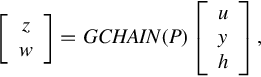
where we denote the GCSR matrix

h is an arbitrary rational vector and ![]() is the Moore-Penrose inverse of P21.
is the Moore-Penrose inverse of P21.
If P21 is invertible, then the CSR [22, 90] exists for the plant P, Eq. (14.4) becomes

where the CSR matrix is

Further denote in Eq. (14.5)

where the sizes of the block matrices G11, G12, G13, G21, G22, G23 are m × p, m × q, m × r, r × p, r × q, r × r, respectively.
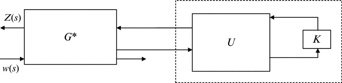
Now consider the terminated cascade connection (14.2) and (14.4) (refer to Fig. 14.1), by denoting Σ = [G21K + G22G23], one can easily obtain a {1}-inverse of Σ, which is important in the sequel.
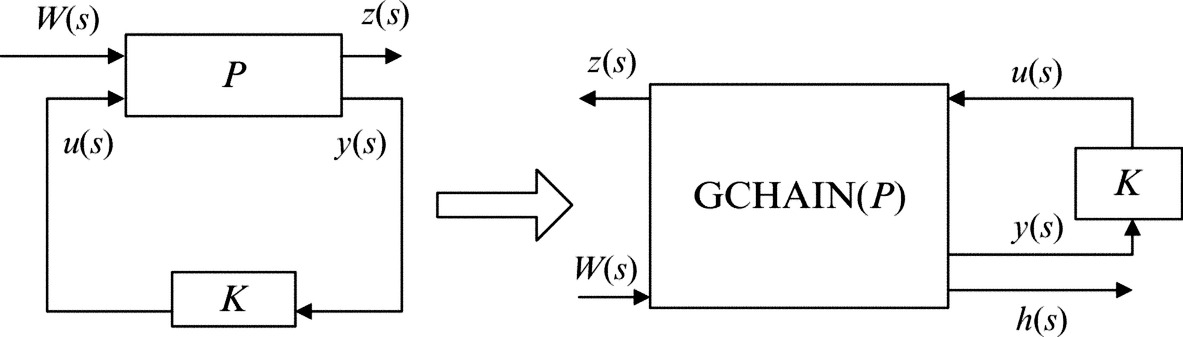 control scheme is reduced to a terminated cascade connection of the generalized chain-scattering representation.
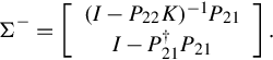
When considering the terminated cascade connection (14.2) and (14.4) (refer to Fig. 14.1), two primary issues that play a key role in our approach need to be considered. One is that the representation (14.4) together with the relation (14.2) can determine [yT, hT]T. It will be seen clearly that this is always the case provided that the closed-loop system is well-posed.
The other issue is termed as output uniqueness, i.e., the condition under which the closed-loop system is able to give rise to a unique output z. These issues are central to the existence of the relevant generalized transfer function [116]. Interestingly, the determined generalized transfer function not only produces a unique output z, being a functional operator, but it is also exactly equal to the linear fractional transformation, once the condition of output uniqueness is satisfied. The following theorems establish the above interesting observations.
Theorem 14.2.2
For the terminated cascade connection (14.2) and (14.4) of the GCSRs, the generalized transfer functions from w to z exist if and only if the condition of output uniqueness
is satisfied. The above condition is equivalent to
Proof
Considering the terminated cascade connection (14.2) and (14.4) of the GCSRs, which is described by [zT, wT]T = G*[uT, yT, hT]T, u = Ky, where G* is given by Eq. (14.5), (14.6), one has
Well-posedness of the closed-loop system means the matrix [P21*(I − P22K) I] is invertible, from the relation

noting that the matrix ![]() is of full row rank, one thus concludes that Σ is of full row rank. Therefore, one can always solve Eq. (14.9) for [yT, hT]T and obtain
is of full row rank, one thus concludes that Σ is of full row rank. Therefore, one can always solve Eq. (14.9) for [yT, hT]T and obtain
where q is any rational vector. Substituting Eq. (14.11) into Eq. (14.10), Eq. (14.10) reads
Hence for Eq. (14.12) to determine the generalized transfer function from w to z, it is sufficient and necessary that the following condition of output uniqueness is satisfied
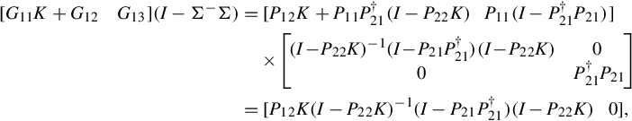
due to the fact that q is arbitrary. One can further verify that the output uniqueness condition (14.13) is equivalent to Eq. (14.7). From Proposition 14.2.1 it follows that

where the relations (i) and (ii) in Definition 14.1.1 are used. Now
where we have used
and
From this we can see that the output uniqueness condition (14.13) is equivalent to Eq. (14.7) for the specially chosen {1}-inverse of Σ given by Proposition 14.2.1. This finishes the proof.
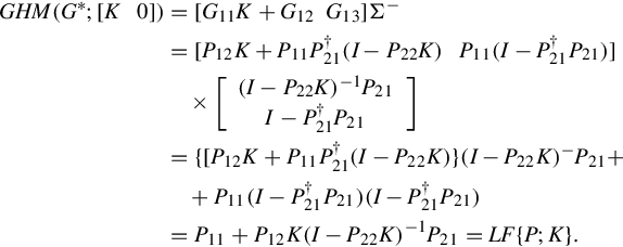
Unlike Kimura’s approach [22, 90] of augmentation in the regular case, in the GCSR matrix the block matrix G23 is of r × r, the matrix [G21K + G22G23] is subsequently of r × (q + r), which is nonsquare and is not invertible. This is one of the reasons that we have to utilize the matrix generalized inverses and where the difficulties arise from the present approach. It is noted that, if the condition of output uniqueness is satisfied, Eq. (14.12) determines a generalized transfer function from w to z, which is given by
where Σ− is given by Proposition 14.2.1. As a matter of fact this generalized transfer function is an extension to the homographic transformation that is used [22, 90] in dealing with the regular ![]() control problem. We therefore term it as the generalized homographic transformation and denote it by GHM(G*;[K 0]) following the notation adopted in [22, 90].
control problem. We therefore term it as the generalized homographic transformation and denote it by GHM(G*;[K 0]) following the notation adopted in [22, 90].
It is of further interest to look at the relationship between the above proposed generalized homographic transformation and the linear fractional transformation. It is interesting that, being a functional operator, the generalized homographic transformation is equal to the linear fractional transformation. This observation is stated as the following theorem.
Theorem 14.2.3
For the terminated cascade connection (14.2) and (14.4), if the output uniqueness s condition is satisfied, then
The above theorems are interesting, not least for the way in which they reduce the original closed-loop system (14.1) and (14.2) into a wave scatter GCHAIN(P) terminated by a load K. This situation is illustrated in Fig. 14.1. More important than this, however, is that the implied mechanism enables us to pose the nonstandard ![]() control problem in the framework of GCSRs in the following manner.
control problem in the framework of GCSRs in the following manner.
Nonstandard ![]() problem reformulation: Find a controller (load) K such that the terminated cascade connection (14.2) and (14.4) (refer to Fig. 14.1) is well-posed, internally stable, the output uniqueness condition is satisfied and
problem reformulation: Find a controller (load) K such that the terminated cascade connection (14.2) and (14.4) (refer to Fig. 14.1) is well-posed, internally stable, the output uniqueness condition is satisfied and
One further observation arising from Theorem 14.2.3 is that the ![]() norm of the closed-loop system can be given equivalently in terms of the generalized homographic transformation. It will also be seen clearly in the next section that the internal stability of the terminated cascade connection (14.2) and (14.4) can be characterized in terms of the A-matrix in the corresponding state-space realization to the generalized homographic transformation. These two observations are exactly the rationale behind the above reformulation of the nonstandard
norm of the closed-loop system can be given equivalently in terms of the generalized homographic transformation. It will also be seen clearly in the next section that the internal stability of the terminated cascade connection (14.2) and (14.4) can be characterized in terms of the A-matrix in the corresponding state-space realization to the generalized homographic transformation. These two observations are exactly the rationale behind the above reformulation of the nonstandard ![]() control problem.
control problem.
14.3 Solvability of nonstandard control problem
This section mainly studies the state-space realization for the generalized homographic transformation and some fundamental cascade structures of the ![]() control systems in the framework of GCSR. Certain sufficient conditions for the solvability of the nonstandard
control systems in the framework of GCSR. Certain sufficient conditions for the solvability of the nonstandard ![]() control problem are then established via
control problem are then established via ![]() -lossless factorization of GCSR.
-lossless factorization of GCSR.
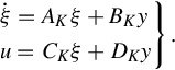
If the state-space realizations for the GCSR and the controller K are given by

and

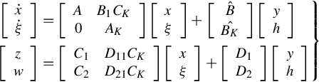
respectively. The above relations (14.16) and (14.17) are then written as
and
Elimination of u from the above relations yields
where we denote

In a similar manner described in [90] and considering the output uniqueness condition, from the above relations one obtains the state-space realization of the generalized homographic transformation GHM(G*;[K 0]) given by

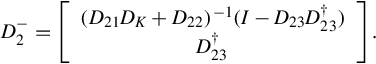
where
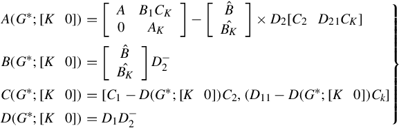
where ![]() is a {1}-inverse of D2 given by
is a {1}-inverse of D2 given by
Now we are ready to introduce the following definition.
Definition 14.3.1
A terminated system (14.2) and (14.4) is said to be internally stable with respect to the generalized homographic transformation GHM(G*;[K 0]) if the corresponding A-matrix A(G*;[K 0]) given in Eq. (14.23) is stable.
For a closed-loop system (14.1) and (14.2), if the CSR [22, 90] exists and is given by

then being the closed-loop transfer function from w to z the usually used linear fractional transformation can be represented [22, 90] as the homographic transformation, i.e.,
It is not difficult to see that, in the case that the CSR exists for the plant P, any generalized homographic transformation comes out to be the homographic transformation, i.e.,
To derive the solvability of the nonstandard ![]() control problem, the following results are crucial.
control problem, the following results are crucial.
Theorem 14.3.1
For the terminated cascade connection (Fig. 14.2) of a GCSR G* = GCHAIN(P1) and a CSRU = CHAIN(P2), if the condition of output uniqueness is satisfied, then we have
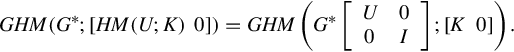
Proof
Let
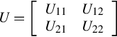
and G* be given by Eq. (14.6), subsequently
From Theorem 14.2.2, the output uniqueness condition for the left-hand side of relation (14.24) is
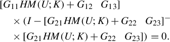
By substituting Eq. (14.25) into Eq. (14.26) and noting
one can see that Eq. (14.26) is equivalent to
which is exactly the output uniqueness condition for the right-hand side of relation (14.24). One therefore has actually proved that the existence of GHM(G*;[HM(U;K) 0]) implies the existency of
and vice versa. The assertion that they are equal follows directly from the fact

This completes the proof.
Theorem 14.3.2
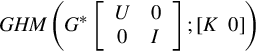
For the terminated cascade connection of a GCSR G*, if the condition of output uniqueness is satisfied, then we have
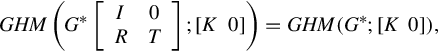
where R and T are any rational matrix with appropriate dimensions and T is nonsingular.
Proof
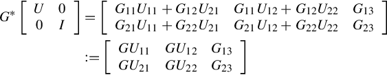
Let G* be given by Eq. (14.6), and according to the partition of G*

by using Theorem 14.2.2 and in a similar manner to the proof of Theorem 14.3.3, we can see that the output uniqueness condition for the left-hand side of relation (14.30) is equivalent to that for the right-hand side. By noting that
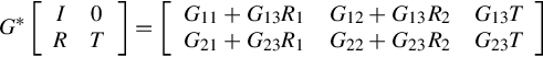
we find that
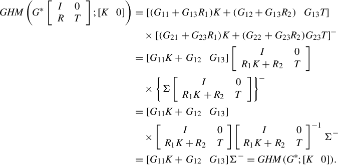
We thus finish the proof.
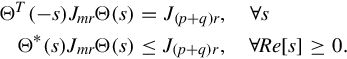
(J, J′)-lossless factorization [22, 90] is a general notion that includes the well-known inner-outer factorization and the spectral factorization. If a matrix ![]() is represented as a product G(s) = Θ(s)Π(s), where
is represented as a product G(s) = Θ(s)Π(s), where ![]() is (Jmr, Jpq)-lossless and Π(s) is unimodular in
is (Jmr, Jpq)-lossless and Π(s) is unimodular in ![]() , then G(s) is said to have a (Jmr, Jpq)-lossless factorization. It is established [22, 90] that the problem of regular
, then G(s) is said to have a (Jmr, Jpq)-lossless factorization. It is established [22, 90] that the problem of regular ![]() control can be reduced to finding a special class of (J, J′)-lossless factorization of the CSR. On the bases of Definition 14.3.1 and Theorems 14.3.1 and 14.3.3, concerning the solvability of the nonstandard
control can be reduced to finding a special class of (J, J′)-lossless factorization of the CSR. On the bases of Definition 14.3.1 and Theorems 14.3.1 and 14.3.3, concerning the solvability of the nonstandard ![]() control problem, we are now ready to propose the following important result.
control problem, we are now ready to propose the following important result.
Theorem 14.3.3
Assume that the GCSR G* = GCHAIN(P) has no zeros or poles on the jω-axis. If the GCSR G* has a (Jmr, J(p+q)r)-lossless factorization
where Π(s) has the form
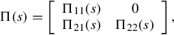
where Π11(s), Π21(s), and Π22(s) are of (p + q) × (p + q), r × (p + q), and r × r, respectively, and if the output uniqueness condition
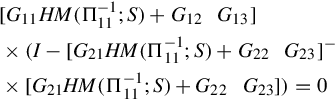
is satisfied, where S is an arbitrary matrix in ![]() , the {1}-inverses can be arbitrary, then the nonstandard d
, the {1}-inverses can be arbitrary, then the nonstandard d ![]() control problem is solvable for the original plant (14.1), the desirable
control problem is solvable for the original plant (14.1), the desirable ![]() controllers are given by
controllers are given by
and the closed-loop transfer function is Φ = HM(Θ;S).
Proof
According to the reformulation of the problem, to prove this statement it is sufficient to see that any desirable controller given by Eq. (14.37) satisfies the output uniqueness condition (14.34) and
if G* has a (Jmr, J(p+q)r)-lossless factorization given by Eq. (14.32) with Π(s) being the specific form described in Eq. (14.33).
As far as the output uniqueness condition (14.34) is concerned, Theorem 14.2.2 tells us that it is a must for the generalized homographic transformations to exist.
From Lemma 4.4 in [90] if the matrix Θ(s) is (J, J′)-lossless, then there exists a lossless matrix P1 such that Θ(s) is a CSR of P1, i.e., Θ(s) = CHAIN(P1). Subsequently, if ![]() , taking into account Theorem 4.15 in [90], then we find that
, taking into account Theorem 4.15 in [90], then we find that

Based on the above observations, by using Theorems 14.3.1 and 14.3.3, it follows that
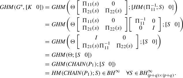
As far as the issue of internal stability is concerned in the above equaling process and considering Definition 14.3.1, one can see that the ![]() controller only cancels out all the stable poles and zeros from the (J, J′)-lossless factorization. The internal stability is therefore left invariant.
controller only cancels out all the stable poles and zeros from the (J, J′)-lossless factorization. The internal stability is therefore left invariant.
Due to the fact that one needs to use Theorem 4.15 of [90] in proposing the above theorem, we have assumed that GCSR G* = GCHAIN(P) has no zeros or poles on the jω-axis. However, this condition is not as restrictive as the standard assumption (A) that we are trying to relax in this approach. To see this, take the following simple example.
Example 14.3.1
Consider the plant
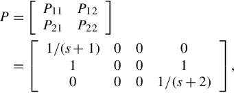
where
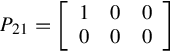
is not of full row rank. The standard assumption (A) is not satisfied by the above plant. It is seen that
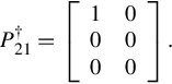
Further calculations yield the GCSR matrix
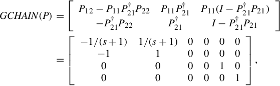
which has no zeros or poles on the imaginary axis.
The invariant zeros or poles of GCSR G* = GCHAIN(P) can be understood in the usual way [5] for a GCSR matrix is still a rational matrix though it is essentially a generalized transfer function [116] of the plant. In the case that the GCSR matrix holds any invariant zero or pole on the imaginary axis one can choose a controller to create a pole or zero in the same point. Then the invariant zero or pole is canceled via pole-zero cancelation. Because of our requirement of internal stability this is only possible for zero or pole in the open left half plane. For zero or pole in the open right half plane it is clearly not possible. In the case of an invariant zero or pole on the imaginary axis we can achieve this cancelation proximately by creating a pole or a zero in the left half plane that is very close to the imaginary axis. A treatment in this manner is given in [126].
It should also be noted that the above triangular structure of the unimodular factor Π(s) in Eq. (14.33) is similar to that of Theorem 7.7 in [90] for the four block cases. In [22], a procedure based on J-lossless conjugation and then formulated in terms of the solutions of two relevant algebraic Riccati equations has already developed, which brings any rational functional matrix G(s) into its (J, J′)-lossless factorization, i.e., G(s) =Θ1(s)Π1(s), where Θ1(s) is (J, J′)-lossless and Π1(s) is unimodular, though Π1(s) is not necessarily in a triangular form. This procedure can also be applied to find the factorization required in the above theorem in the following manner. One first obtains the above (J, J′)-lossless factorization
by using Kimura’s approach, and then computing the LU decomposition of Π1(s) by the row − echelon factoring method to obtain the required triangular form. In more detail, considering Π1(s) is a unimodular matrix, one finds a special LU decomposition such that Π1(s) = L(s)U(s), where the row-echelon factoring matrix L(s) can be expected to be orthogonal, and U(s) is in the required triangular form. Note that, in this case the matrix Θ(s) =Θ1(s)L(s) is still (J, J′)-lossless for it satisfies [22]
For the techniques of traditional LU decomposition and a modified LU decomposition of a rational function matrix, we can refer to [127]. For numerical symbolic computation, Maple has provided a routine LUdecomp for this purpose. A remaining interesting topic worthy of further research, however, is to show how this kind of special triangular structure can be directly linked to certain algebraic Riccati equations.
The above theorem is interesting in that it generalizes the result proposed by Kimura [22, 90] from the regular case to the nonstandard case. It establishes a close tie between the nonstandard ![]() control problem and (J, J′)-lossless factorization by displaying the fact that, just as in the regular problem, if the unimodular part of a GCSR is completely canceled out by the controller and a certain output uniqueness condition is satisfied, then this nonstandard problem is solvable.
control problem and (J, J′)-lossless factorization by displaying the fact that, just as in the regular problem, if the unimodular part of a GCSR is completely canceled out by the controller and a certain output uniqueness condition is satisfied, then this nonstandard problem is solvable.
14.4 Conclusions
We have presented a GCSR approach to the nonstandard ![]() control problem. Certain sufficient conditions for the solvability of this problem are established via a (J, J′)-lossless factorization of GCSR. These results thus present extensions to Kimura’s results on the CSR approach to
control problem. Certain sufficient conditions for the solvability of this problem are established via a (J, J′)-lossless factorization of GCSR. These results thus present extensions to Kimura’s results on the CSR approach to ![]() control. The suggested approach is believed to be workable in the practical control setting due to the fact that some computational formulas and procedures of the Moore-Penrose inverse of a matrix are available through the work of Klema and Laub [128], which can be applied to obtain the GCSR, and the J-lossless conjugation approach [22, 90] has provided a powerful tool for computing the required (J, J′)-lossless factorization of the GCSR. Future research would focus on the issue of how these solution conditions in terms of the GCSR of the plant can be directly linked to the relevant algebraic Riccati equations in a state-space scheme.
control. The suggested approach is believed to be workable in the practical control setting due to the fact that some computational formulas and procedures of the Moore-Penrose inverse of a matrix are available through the work of Klema and Laub [128], which can be applied to obtain the GCSR, and the J-lossless conjugation approach [22, 90] has provided a powerful tool for computing the required (J, J′)-lossless factorization of the GCSR. Future research would focus on the issue of how these solution conditions in terms of the GCSR of the plant can be directly linked to the relevant algebraic Riccati equations in a state-space scheme.