
Realization of behavior
Abstract
This chapter presents a new notion of realization of behavior. It has been shown that realization of behavior generalizes the classical concept of realization of transfer function matrix. The basic idea in this approach is to find an autoregressive moving-average (ARMA) representation for a given frequency behavior description such that the known frequency behavior is completely recovered to the corresponding dynamical behavior. From this point of view, realization of behavior is seen to be a converse procedure to the latent variable eliminating process. Such a realization approach is believed to be highly significant in modeling a dynamical system in some real cases where the system behavior is conveniently described in the frequency domain. Since no numerical computation is needed, the realization of behavior is believed to be particularly suitable for situations in which the coefficients are symbolic rather than numerical.
Based on this idea, the behavior structures of the generalized chain-scattering representation (GCSR) and the dual generalized chain-scattering representation (DGCSR) have been clarified. It has been shown that any GCSR or any DGCSR develops the same (frequency) behavior. Subsequently the corresponding ARMA representations are proposed and are proved to be realizations of behavior for any GCSR and any DGCSR. More specifically, two Rosenbrock PMDs are found to be the realizations of behavior for any GCSR.
Keywords
Realization of behavior; Transfer function matrix; Autoregressive moving-average (ARMA); Latent variable eliminating process; Chain-scattering representation (CSR); Generalized chain-scattering representation (GCSR); Dual generalized chain-scattering representation (DGCSR); Polynomial matrix description (PMD); Infinite-dimensional systems
12.1 Introduction
In classical network theory, a circuit representation called the chain matrix [21] was widely used to deal with the cascade connection of circuits arising in analysis and synthesis problems. Based on this, Kimura [22] developed the chain-scattering representation (CSR), which was subsequently used to provide a unified framework for ![]() control theory. Kimura’s approach is, however, only available to the special cases where the matrices P21 and P12 (refer to Eq. 11.1) satisfy some assumptions of full rank. Recently, in [31] this approach was extended to the general case in which such conditions are essentially relaxed. From an input-output consistency point of view, the generalized chain-scattering representation (GCSR) and the dual generalized chain-scattering representation (DGCSR) emerge and are there successfully used to characterize the cascade structure property and the symmetry of general plants in a general setting.
control theory. Kimura’s approach is, however, only available to the special cases where the matrices P21 and P12 (refer to Eq. 11.1) satisfy some assumptions of full rank. Recently, in [31] this approach was extended to the general case in which such conditions are essentially relaxed. From an input-output consistency point of view, the generalized chain-scattering representation (GCSR) and the dual generalized chain-scattering representation (DGCSR) emerge and are there successfully used to characterize the cascade structure property and the symmetry of general plants in a general setting.
Latterly behavioral theory (see, e.g., [26, 27]) has received broad acceptance as an approach for modeling dynamical systems. One of the main features of the behavioral approach is that it does not use the conventional input-output structure in describing systems. Instead, a mathematical model is used to represent the systems in which the collection of time trajectories of the relevant variables are viewed as the behavior of the dynamical systems. This approach has been shown [26, 28] to be powerful in system modeling and analysis. In contrast to this, the classical theories such as Kalman’s state-space description and Rosenbrock’s polynomial matrix description (PMD) take the input-output representation as their starting point. In many control contexts it has proven to be very convenient to adopt the classical input/state/output framework. It is often found that the system models, in many situations, can easily be formulated into the input/state/output models such as the state space descriptions and the PMDs. Based on such input/state/output representations, the action of the controller can usually be explained in a very natural manner and the control aims can usually be attained very effectively.
As far as the issue of system modeling is concerned the computer-aided procedure, i.e., the automated modeling technology, has been well developed as a practical approach over recent years. If the physical description of a system is known, the automated modeling approach can be applied to find a set of equation to describe the dynamical behavior of the given system. It is seen that, in many cases, such as in an electrical circuit or, more generally, in an interconnection of blocks, such a physical description is more conveniently specified through the frequency behavior of the system. Consequently in these cases, a more general theoretic problem arises, i.e., if the frequency behavior description of a system is known, what is the corresponding dynamical behavior? In other words, what is the input/output or input/state/output structure in the time domain that generates the given frequency domain description. It turns out that this question can be interpreted through the notion of realization of behavior, which we shall introduce in this chapter.
In fact, as we shall see later, realization of behavior, in many cases, amounts to introduction of latent variables in the time domain. From this point of view, realization of behavior can be understood as a converse procedure of the latent variable elimination theorem [27] in one way or another. It should be emphasized that realization of behavior also generalizes the notion of transfer function matrix realization in the classical control theory framework, as the behavior equation is a more general description than the transfer function matrix. As a special case, the behavior equations determine a transfer matrix of the system if they represent an input-output system [27, 29], i.e., when the matrices describing the system satisfy a full rank condition.
Recently in [30], a realization approach was suggested that reduces high-order linear differential equations to the first-order system representations by using the method of “linearization.” From the point of view of realization in a physical sense one is, however, forced to start from the system frequency behavior description into which system behavior is generally described rather than from the high-order linear differential equations in time domain. Also a constructive procedure for autoregressive (AR) equation realization has been introduced in [114].
One of the main aims of this chapter is to present a new notion of realization of behavior. Further to the results of [31], the input-output structure of the GCSRs and the DGCSRs are thus clarified by using this approach. Subsequently the corresponding autoregressive-moving-average (ARMA) representations are proposed and are proved to be realizations of behavior for any GCSR and for any DGCSR. Once these ARMA representations are proposed, one can further find the corresponding first-order system representations by using the method of [30] or other well-developed realization approaches such as Kailath [32].
These results are interesting in that they provide a good insight into the natural relationship between the (frequency) behavior of any GCSR and any DGCSR and the (dynamical) behavior of the corresponding ARMA representations. Since no numerical computation is involved in this approach, realization of behavior is particularly accessible for situations in which the coefficient are symbolic rather than numerical. Based on the realization of behavior, one can further find the corresponding first-order system representations by using the classical realization approaches [30, 32]. Also a constructive procedure for AR equation realization suggested by Vafiadis and Karcanias [114] can be used to obtain the required first-order system representations.
The following result can be easily proposed and can be easily proved by using the definition of 1-inverse of a polynomial matrix. It is presented here for later use.
12.2 Behavior realization
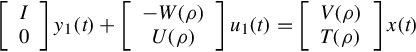
This section introduce the concept of realization of behavior. Recall that in the behavioral framework the (dynamical) behavioral equations of an ARMA representation [27] are
where ![]() stands for the external variables representing the dynamical behavior of the underlying dynamical system, ξ(t) which are called latent variables corresponding to auxiliary variables resulting from the modeling procedure. R1(ρ), R2(ρ) and S(ρ) are polynomial matrices containing the differential operator ρ = d/dt. In order to distinguish them from the existing notation y, u of Eq. (11.1), the external variables are denoted by y1 and u1. When S(ρ) = 0, Eq. (12.1) is termed [27] an AR representation.
stands for the external variables representing the dynamical behavior of the underlying dynamical system, ξ(t) which are called latent variables corresponding to auxiliary variables resulting from the modeling procedure. R1(ρ), R2(ρ) and S(ρ) are polynomial matrices containing the differential operator ρ = d/dt. In order to distinguish them from the existing notation y, u of Eq. (11.1), the external variables are denoted by y1 and u1. When S(ρ) = 0, Eq. (12.1) is termed [27] an AR representation.
In the following approach we are interested in the external behavior of the system (12.1), where we choose the underlying function space to be ![]() , this function space consists of all the infinitely differentiable functions that are defined for all time
, this function space consists of all the infinitely differentiable functions that are defined for all time ![]() and take values in the real number field
and take values in the real number field ![]() . For brevity, we write
. For brevity, we write ![]() . Then the dynamical external behavior of Eq. (12.1) is given by
. Then the dynamical external behavior of Eq. (12.1) is given by
From the above, to avoid the trivial case that the external behavior is empty, i.e., to ensure that there exist latent variables, every pair (y1(t), u1(t)) in the external behavior must be consistent, that is

where {1}-inverse is arbitrary. It is immediately noted that, when S(ρ) is invertible or more specially when S(ρ) = I, the above condition is automatically satisfied.
In many real cases (for example, electrical circuits), however, system behavior is usually described (see Example 12.2.1) in the frequency domain as
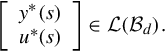
where ![]() , and
, and ![]() as the following example suggests, are not polynomial but rational matrices. The vector-valued signals u*(s), y*(s), and η(s) live in the square (Lebesgue) integrable functional spaces
as the following example suggests, are not polynomial but rational matrices. The vector-valued signals u*(s), y*(s), and η(s) live in the square (Lebesgue) integrable functional spaces ![]() , and
, and ![]() respectively.
respectively.
Example 12.2.1
Consider the system. The loop equations of Fig. 12.1 are written as
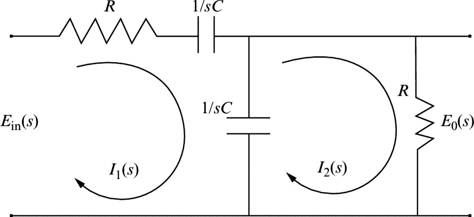

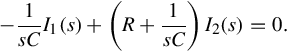
In order to obtain the transfer function ![]() , one needs to solve for I2(s) to obtain
, one needs to solve for I2(s) to obtain
and then note that the output voltage is
This suggests that I1(s) can be regarded as latent variable, the original loop equations thus can be written into

which is just in the form of Eq. (12.3). The coefficient matrices of the external variables and the latent variables are seen to be rational but not necessarily polynomial.
As a special case when C(s) = 0 and B(s) is invertible, Eq. (12.3) determines a transfer function G(s) = −B−1(s)A(s).
The frequency behavior of Eq. (12.3) is given by
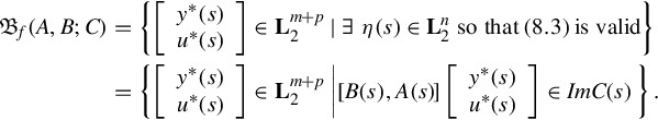
In here the matrix B(s) is not necessarily invertible. It will be seen later that this is the reason why the realization of behavior comes out to be a generalization of realization of transfer function. Instead of this condition, we only make a relaxed assumption that every u* in the behavior is consistent, i.e.,
where B−(s) is any {1}-inverse of B(s). Again it should be noted that, when B(s) is invertible or more specially when B(s) = I, the above condition is automatically satisfied. By denoting

where ![]() denotes the Laplace transformation of f(t), the definition of realization of behavior follows.
denotes the Laplace transformation of f(t), the definition of realization of behavior follows.
Definition 12.2.1
Given a frequency behavior description (Eq. 12.3), if there exists an ARMA representation (Eq. 12.1), i.e., there exist polynomial matrices R1(ρ), R2(ρ), and S(ρ) such that
then the ARMA representation (Eq. 12.1) is said to be a realization of behavior for Eq. (12.3).
Remark 12.2.1
It should be noted that, in the frequency behavior description (Eq. 12.3), the matrices A(s) and B(s) are assumed to be rational, not necessarily polynomial. If they are polynomial, it is obvious that the following AR representation [27]
is a realization of behavior for Eq. (12.3). In this case, one does not need to introduce any latent variable.
Remark 12.2.2
The above concept is a generalization to the classical notion of realization of transfer function matrix.
To see this, let us consider the special case, when B(s) is invertible and C(s) = 0. Then Eq. (12.3) determines a transfer matrix and can be written as
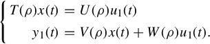
If there exist polynomial matrices T(ρ), U(ρ), V (ρ), and W(ρ) of appropriate dimensions such that T(ρ) is invertible and
then by Definition 12.2.1, it is easy to verify that the following ARMA representation
is a realization of behavior for the frequency behavior description (Eq. 12.3). It is noted that Eq. (12.10) is nothing but the Rosenbrock PMD
The condition of consistency is seen to be satisfied because of the invertibility of T(ρ).
When T(ρ) = ρE − A with E singular, the above PMD is termed a singular system, while when T(ρ) = ρI − A, the above description is known as the conventional state space system. It is clearly seen that in the above special cases, realization of behavior is equivalent to realization of transfer function in the classical sense.
12.3 Realization of behavior for GCSRs and DGCSRs
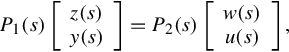
Before developing the realization of behavior for GCSRs, we will establish a realization of behavior for the general plant. Given the general plant described by

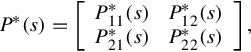
where Pij(s) (i = 1, 2; j = 1, 2) are all rational matrices with dimensions mi × kj (i = 1, 2; j = 1, 2), consider the rational matrix ![]() . It is well-known [4] that there always exist nonunique polynomial pairs
. It is well-known [4] that there always exist nonunique polynomial pairs ![]() and
and ![]() such that
such that
It should be noted in here P1(s) and P2(s) do not need to be coprime. In this way, the following result is obtained.
Theorem 12.3.1
The following AR representation
is a realization of behavior for the general plant (Eq. 12.11), where the external variables are denoted by
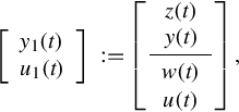
and the polynomial matrices P1(ρ), P2(ρ) satisfy Eq. (12.12).
Proof
Under the decomposition (Eq. 12.12), Eq. (12.11) can be written into
the above frequency behavior is seen to be ![]() while the dynamical external behavior of the AR representation (Eq. 12.13) is
while the dynamical external behavior of the AR representation (Eq. 12.13) is

Now let

The Laplace transformation of Eq. (12.13) with zero initial condition yields
where ![]() Thus Eq. (8.14) gives
Thus Eq. (8.14) gives
Hence the theorem follows from Definition 12.2.1.
Recall now Theorem 11.2.2. If the input-output pair (u(s), y(s)) is consistent about w to the plant P, then the GCSR is represented by

where we denote the GCSR matrix

The above GCSR gives rise to the frequency behavior

It can be proved that every GCSR gives rise to the same frequency behavior, in other words, the frequency behavior of GCSRs is independent of the particular {1}-inverse. The following theorem establishes this observation.
Theorem 12.3.2
Given any two GCSEs GCHAIN(P;P21−), ![]() , which are formulated in terms of two {1}-inverse of P21 respectively, one has
, which are formulated in terms of two {1}-inverse of P21 respectively, one has
From Lemma 11.1.2, there exists a matrix K(s) such that
Also the input-output pair (u(s), y(s)), if being consistent to the plant P, must satisfy (Theorem 11.2.1)

This follows that
Given any

there should be a rational vector h1(s) such that

By substituting Eqs. (12.16), (12.17) into Eq. (12.18), one yields
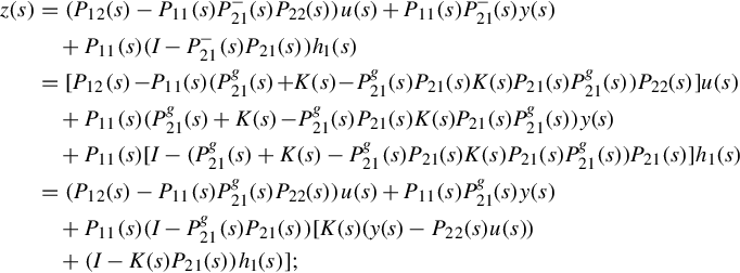

By letting
the above formulations about z(s) and w(s) can be written into the following matrix form

which displays the fact that

Subsequently
This finishes the proof.
By the virtue of the above theorem, the frequency behavior of any GCSR thus can be simply denoted by ![]()
One of the remaining aims of this section is to show how the frequency behavior of GCSRs can be realized as the dynamical behavior of an ARMA representation through the approach of realization of behavior. To this end, the general plant (Eq. 12.11) is rewritten into

where g(s) is the least common (monic) multiple of the denominator polynomials of all the entries in P(s), and Pij*(s)/g(s) = Pij(s), i = 1, 2; j = 1, 2. It is immediately noted that the above decomposition of P is a special case of Eq. (12.12). By letting

where ![]() is the identity matrix with dimension m1 + m2. Eq. (12.19) thus takes the form
is the identity matrix with dimension m1 + m2. Eq. (12.19) thus takes the form

It should be noted that in here P*(s) is a polynomial matrix and g(s) is a polynomial.
As is shown before, the realization of behavior for a general plant is rather straightforward, while the realization of behavior for GCSR is more obscure, as in this case the introduction of latent variables is necessary. To propose a realization of behavior for GCSRs, consider the following ARMA representation
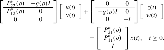
The above ARMA representation is in fact

where all the identity matrices and all the zero block matrices are of appropriate dimensions. ![]() are the latent variables. It is noted that every condition pair
are the latent variables. It is noted that every condition pair

is consistent about the latent variables x(t) is equivalent that every input-output pair (u(s), y(s)) is consistent about w.
The following technical result will be used in the proof of Theorem 12.3.3. It is stated as a lemma.
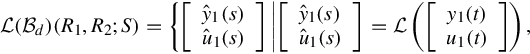
Lemma 12.3.1
Let all the initial conditions and their derivatives of u(⋅) and y(⋅) be zero. The following condition of consistency in the time domain
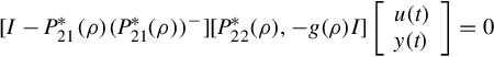
is equivalent to the following consistency condition in the frequency domain
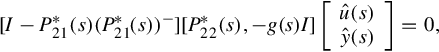
i.e.,

where ![]() ,
, ![]() denote the Laplace transformation of u(t) and y(t) respectively.
denote the Laplace transformation of u(t) and y(t) respectively.
Now we are ready to state and prove the following result.
Proof
Given any GCSR, its frequency behavior is ![]() . The dynamical external behavior of the ARMA representation (Eq. 12.23) is
. The dynamical external behavior of the ARMA representation (Eq. 12.23) is
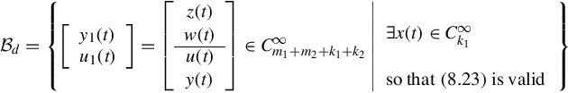
 , to ensure that there exists x(t) such that Eq. (12.23), i.e., Eq. (12.24) is valid, u1(t) must be consistent to Eq. (12.24). This suggests that

It is easily seen to be equivalent to

The Laplace transformation of Eq. (12.24) (with zero initial conditions) yields
and

where ![]() Due to the reason stated in the proof of Theorem 12.3.1 all the Laplace transformed initial vectors that are associated with the initial values of the variables and their derivatives are zeros.
Due to the reason stated in the proof of Theorem 12.3.1 all the Laplace transformed initial vectors that are associated with the initial values of the variables and their derivatives are zeros.
Due to the consistency of  , Eq. (12.26) determines the latent variables
 ![]() . By solving the latent variables
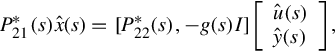
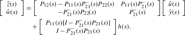
. By solving the latent variables ![]() in Eq. (12.26) and then substituting into Eq. (12.27), one obtains
in Eq. (12.26) and then substituting into Eq. (12.27), one obtains

where h(s) is any rational vector. By noticing that Pij*(s) = g(s)Pij(s), i = 1, 2; j = 1, 2, and that P21−(s) = g(s)(P21*)−(s), Eq. (12.28) can also be written into
It is thus seen that
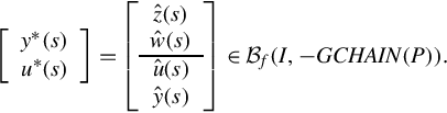
So far it has been proved that
To prove the statement
let

there should be a rational vector h1(s) such that
for any {1}-inverse of P21. Furthermore, the input-output pair (u(s), y(s)) must be consistent to the plant P. Now let
using the consistency of (u(s), y(s)), it is easy to verify that the variables y*, u*, and x satisfy Eqs. (12.26), (12.27), this is to say that
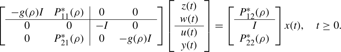
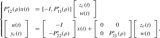
On noticing Eq. (12.20), one can write the ARMA representation (Eq. 12.23) into the following Rosenbrock PMD
It is easily seen that
By substituting the above and
into the GCSR

using the notations of zc(s) = g(s)z(s) and yc(s) = g(s)y(s), one can find that

where we denote the matrix
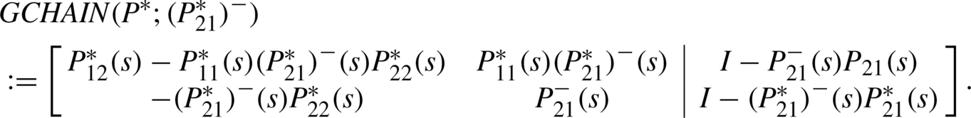
A further result concerning the realization of behavior for any GCSR GCHAIN(P*; (P21*)−) is the following theorem.
Proof
This follows readily from Theorem 12.3.3 on noting that
where h(s) is arbitrary rational vector, and that in the matrix P* the least common (monic) multiple of the denominator polynomials of all the entries is 1.
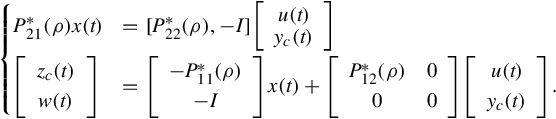
The realization of behavior for DGCSRs of the plant P can be proposed in a completely analogous manner. To this end, consider the following ARMA representation
 (12.32)
The above ARMA representation is in fact

Also if Eq. (12.32) is written into the following Rosenbrock PMD
one proposes a realization of behavior for any DGCSR DGCHAIN(P*;(P21*)−), where any DGCHAIN(P*;(P12*)−) is given by

and satisfies
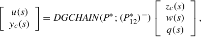
where q(s) is arbitrary rational vector. (P12*)−(s) is any {1}-inverse of P12*(s). This result is stated in the following theorem.
12.4 Conclusions
This chapter has presented a new notion of realization of behavior. It has been shown that realization of behavior generalizes the classical concept of realization of transfer function matrix by virtue of the input consistency assumption essentially relaxing the condition of full rank, which is put on the relevant matrix to ensure the existence of the transfer function. The basic idea in this approach is to find an ARMA representation for a given frequency behavior description such that the known frequency behavior is completely recovered from the corresponding dynamical behavior. From this point of view, realization of behavior is seen to be a converse procedure to the latent variable elimination process that was studied by Willems [27]. Such a realization approach is believed to be highly significant in modeling dynamical systems in some real cases where the system behavior is conveniently described in the frequency domain. Since no numerical computation is needed, the realization of behavior is believed to be particularly suitable for situations in which the coefficients are symbolic rather than numerical.
From an input/output viewpoint, a CSR is in fact an alternative form of system description. It is well-known and is widely used in classical circuit theory. This approach when combined with the theory of J-spectral factorization provides the most compact theory for ![]() control. CSR is undoubtedly a potential research area due to the fact that it finds many applications in circuit theory,
control. CSR is undoubtedly a potential research area due to the fact that it finds many applications in circuit theory, ![]() control, behavior control, and infinite-dimension system theory. This chapter has investigated the input/output structure of the GCSR and has made contributions regarding this fundamental issue. Based on the approach of realization of behavior, the behavior structures of the GCSRs and the DGCSRs have been clarified. It has been shown that any GCSR or any DGCSR develops the same (frequency) behavior. Subsequently the corresponding ARMA representations are proposed and are proved to be realizations of behavior for any GCSR and for any DGCSR. More specifically, two Rosenbrock PMDs are found to be the realizations of behavior for any GCSR GCHAIN(P*;(P21*)−) and any DGCSR DGCHAIN(P*;(P12*)−). Once these ARMA representations are proposed, one can further find the corresponding first-order system representations by using the method of [30] or other well-developed realization approaches such as Kailath [32]. Also a constructive procedure for AR equation realization suggested by Vafiadis and Karcanias [114] can be used to obtain the required first-order system representations. The results are thus interesting in that they provide a natural linkage between the new chain-scattering approach and the well-developed Rosenbrock PMD theory or the developing behavior theory.
control, behavior control, and infinite-dimension system theory. This chapter has investigated the input/output structure of the GCSR and has made contributions regarding this fundamental issue. Based on the approach of realization of behavior, the behavior structures of the GCSRs and the DGCSRs have been clarified. It has been shown that any GCSR or any DGCSR develops the same (frequency) behavior. Subsequently the corresponding ARMA representations are proposed and are proved to be realizations of behavior for any GCSR and for any DGCSR. More specifically, two Rosenbrock PMDs are found to be the realizations of behavior for any GCSR GCHAIN(P*;(P21*)−) and any DGCSR DGCHAIN(P*;(P12*)−). Once these ARMA representations are proposed, one can further find the corresponding first-order system representations by using the method of [30] or other well-developed realization approaches such as Kailath [32]. Also a constructive procedure for AR equation realization suggested by Vafiadis and Karcanias [114] can be used to obtain the required first-order system representations. The results are thus interesting in that they provide a natural linkage between the new chain-scattering approach and the well-developed Rosenbrock PMD theory or the developing behavior theory.