4.6 Poles and zeros

The connections between a coprime polynomial fraction description for a strictly proper rational transfer function G(s) and minimal realizations of G(s) can be used to define notions of poles and zeros of G(s) that generalize the familiar notions for scalar transfer functions. In addition we characterize these concepts in terms of response properties of a minimal realization of G(s). For the peer results for discrete time, some translation and modification of these results are required.

Given coprime polynomial fraction descriptions

$\begin{array}{l}\hfill G(s)=N(s)D^{-1}(s)=D_L^{-1}(s)N_L(s),\end{array}$

it follows from Theorem 4.3.5 that the polynomials $detD(s)$ and $det{D}_L(s)$ have the same roots. Furthermore from Theorem 4.2.4 it is clear that these roots are the same for every coprime polynomial description. This permits the introduction of terminology in terms of either a right or left polynomial fraction description, though we adhere to a societal bias and use right.

This terminology is compatible with customary usage in the m = p = 1 case. Specifically if s₀ is a pole of G(s), then some entry G_ij(s) is such that $|G_{ij}(s_0)|=\infty .$ Conversely if some entry of G(s) has infinite magnitude when evaluated at the complex number s₀, then s₀ is a pole of G(s). A linear state equation with transfer function G(s) is uniformly bounded-input, bounded-output stable if and only if all poles of G(s) have negative real parts, that is, all roots of $detD(s)$ have negative real parts.

The relation between eigenvalues of A in the linear state equation (4.43) and poles of the corresponding transfer function

$\begin{array}{l}\hfill G(s)=C{(sI-A)}^{-1}B\end{array}$

is a crucial feature in some of our arguments. Writing G(s) in terms of a coprime right polynomial fraction description gives

$\begin{array}{l}\hfill \frac{N(s)\cdot adjD(s)}{detD(s)}=\frac{C[adj(sI-A)]B}{det(sI-A)}.\end{array}$

Using Lemma 4.5.1, Eq. (4.69) reveals that if s₀ is a pole of G(s) with multiplicity σ₀, then s₀ is an eigenvalue of A with multiplicity at least σ₀. But simple single-input, single-output examples confirm that multiplicities can be different, and in particular an eigenvalue of A might not be a pole of G(s). The remedy for this displeasing situation is to assume 4.43 is controllable and observable. Then Eq. (4.69) shows that, since the denominator polynomials are identical up to a constant multiplier, the set of poles of G(s) is identical to the set of eigenvalues of a minimal realization of G(s).

This discussion leads to an interpretation of a pole of a transfer function in terms of zero-input response properties of a minimal realization of the transfer function.

Of course if s₀ is a real pole of G(s), then Eq. (4.70) directly gives a corresponding zero-input response property of minimal realizations of G(s). If s₀ is complex, then the real initial state $x_0+{\overline{x}}_0$ gives an easily computed real response that can be written as a product of an exponential with exponent (Re [s₀])t and a sinusoid with frequency Im [s₀].

The concept of a zero of a transfer function is more delicate. For a scalar function G(s) with coprime numerator and denominator polynomials, a zero is a complex number s₀ such that G(s₀) = 0. Evaluations of a scalar G(s) at particular complex numbers can result in a zero or nonzero complex value, or can be undefined (at a pole). These possibilities multiply for multiinput, multioutput systems, where a corresponding notion of a zero is a complex s₀ where the matrix G(s₀) “loses rank.”

To carefully define the concept of a zero, the underlying assumption we make is that $\mathrm{rank}G(s)=min[m,p]$ for almost all complex values of s. (By “almost all” we mean “all but a finite number.”) In particular, at poles of G(s) at least one entry of G(s) is ill-defined, and so poles are among those values of s ignored when checking rank. (Another phrasing of this assumption is that G(s) is assumed to have rank $min[m,p]$ over the field of rational functions, a more sophisticated terminology that we do not further employ.) Now consider coprime polynomial fraction descriptions

$\begin{array}{l}\hfill G(s)=N(s)D^{-1}(s)=D_L^{-1}(s)N_L(s)\end{array}$

for G(s). Since both D(s) and D_L(s) are nonsingular polynomial matrices, assuming $\mathrm{rank}G(s)=min[m,p]$ for almost all complex values of s is equivalent to assuming $\mathrm{rank}N(s)=min[m,p]$ for almost all complex values of s, and also equivalent to assuming $\mathrm{rank}{N}_L(s)=min[m,p]$ for almost all complex values of s. The agreeable feature of polynomial fraction descriptions is that N(s) and N_L(s) are well-defined for all values of s. Either right or left polynomial fractions can be adopted as the basis for defining transfer-function zeros.

This reduces to the customary definition in the single-input, single-output ease. But a look at multiinput, multioutput examples reveals subtleties in the concept of transmission zero.

Another complication arises as we develop a characterization of transmission zeros in terms of identically zero response of a minimal realization of G(s) to a particular initial state and particular input signal. Namely with m ≥ 2 there can exist a nonzero m × 1 vector U(s) of strictly proper rational functions such that G(s)U(s) = 0. In this situation multiplying all the denominators in U(s) by the same nonzero polynomial in s generates whole families of inputs for which the zero-state response is identically zero. This inconvenience always occurs when m > p. Here we add an assumption that forces m ≤ p.

The basic idea is to devise an input U(s) such that the zero-state response component contains exponential terms due solely to poles of the transfer function, and such that these exponential terms can be canceled by terms in the zero-input response component.

On the other hand suppose s₀ is not a pole of G(s). Using the easily verified identity

$\begin{array}{l}\hfill {(s_{0}I-A)}^{-1}{(s-s_0)}^{-1}={(sI-A)}^{-1}{(s_{0}I-A)}^{-1}+{(sI-A)}^{-1}{(s-s_0)}^{-1},\end{array}$

we can write, for any m × 1 complex vector u₀ and corresponding n × 1 complex vector x₀ = (s₀I−A)⁻¹Bu₀, the Laplace transform expression

$\begin{array}{l}\hfill \begin{array}{cc}& \mathcal{L}\{C{e}^{At}{x}_0+{\int }_0^{t}C{e}^{A(t-\sigma )}B{u}_0{e}^{s_0\sigma }d\sigma \}\\ & =C{(sI-A)}^{-1}{x}_0+C{(sI-A)}^{-1}B{u}_0{(s-s_0)}^{-1}\\ & =C[{(sI-A)}^{-1}{(s_{0}I-A)}^{-1}+{(sI-A)}^{-1}{(s-s_0)}^{-1}]B{u}_0\\ & =G(s_0)u_0{(s-s_0)}^{-1}\\ & =N(s_0)D^{-1}(s_0)u_0{(s-s_0)}^{-1}.\\ \end{array}\end{array}$

Taking the inverse Laplace transform gives, for the particular choice of x₀ above,

$\begin{array}{l}\hfill C{e}^{At}{x}_0+{\int }_0^{t}C{e}^{A(t-\sigma )}B{u}_0{e}^{s_0\sigma }d\sigma =N(s_0)D^{-1}(s_0)u_0{e}^{s_{0}t},t\ge 0.\end{array}$

Clearly the m × 1 vector u₀ can be chosen so that this expression is zero for t ≥ 0 if rank N(s₀) < m, that is, if s₀ is a transmission zero of G(s).

Of course if a transmission zero s₀ is real and not a pole, then we can take u₀ real, and the corresponding x₀ = (s₀I−A)⁻¹Bu₀ is real. Then Eq. (4.74) shows that the complete response for x(0) = x₀ and $u(t)=u_0{e}^{s_{0}t}$ is identically zero. If s₀ is a complex transmission zero, then specification of a real input and real initial state that provides identically zero response is left as a mild exercise.

4.7 State feedback

Properties of linear state feedback

$\begin{array}{l}\hfill u(t)=Kx(t)+Mr(t)\end{array}$

applied to a linear state equation (4.43). As noted, a direct approach to relating the closed-loop and plant transfer functions is unpromising in the case of state feedback. However, polynomial fraction descriptions and an adroit formulation lead to a way around the difficulty.

We assume that a strictly proper rational transfer function for the plant is given as a coprime right polynomial fraction G(s) = N(s)D⁻¹(s) with D(s) column reduced. To represent linear state feedback, it is convenient to write the input-output description

$\begin{array}{l}\hfill Y(s)=N(s)D^{-1}(s)U(s)\end{array}$

as a pair of equations with polynomial matrix coefficients

$\begin{array}{ll}\hfill & D(s)\xi (s)=U(s),\hfill \\ \hfill & Y(s)=N(s)\xi (s).\hfill \end{array}$

The m × 1 vector ξ(s) is called the pseudo-state of the plant. This terminology can be motivated by considering a minimal realization of the form (4.55) for G(s). From Eq. (4.57) we write

$\begin{array}{l}\hfill \begin{array}{cc}\psi (s)\xi (s)& =\psi (s)D^{-1}(s)U(s)\\ & ={(sI-A_0+B_0{D}_{hc}^{-1}{D}_l)}^{-1}{B}_0{D}_{hc}^{-1}U(s)\\ \end{array}\end{array}$

or

$\begin{array}{l}\hfill s\psi (s)\xi (s)=(A_0-B_0{D}_{hc}^{-1}{D}_l)\psi (s)\xi (s)+B_0{D}_{hc}^{-1}U(s).\end{array}$

Defining the n × 1 vector x(t) as the inverse Laplace transform

$\begin{array}{l}\hfill x(t)={\mathcal{L}}^{-1}[\psi (s)\xi (s)],\end{array}$

we see that Eq. (4.81) is the Laplace transform representation of the linear state equation (4.55) with zero initial state. Beyond motivation for terminology, this development shows that linear state feedback for a linear state equation corresponds to feedback of ψ(s)ξ(s) in the associated pseudo-state representation (4.79).

Now, as illustrated in Fig. 4.1, consider linear state feedback for Eq. (4.79) represented by

$\begin{array}{l}\hfill U(s)=K\psi (s)\xi (s)+MR(s),\end{array}$

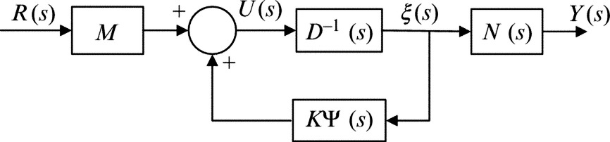
where K and M are real matrices of dimensions m × n and m × m, respectively. We assume that M is invertible. To develop a polynomial fraction description for the resulting closed-loop transfer function, substitute Eq. (4.82) into Eq. (4.79) to obtain

$\begin{array}{l}\hfill \begin{array}{cc}[D(s)-K\psi (s)]\xi (s)& =MR(s)\\ Y(s)& =N(s)\xi (s).\end{array}\end{array}$

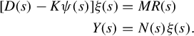
Nonsingularity of the polynomial matrix D(s) − Kψ(s) is assured, since its column degree coefficient matrix is the same as the assumed-invertible column degree coefficient matrix for D(s). Therefore we can write

$\begin{array}{l}\hfill \begin{array}{cc}\xi (s)& ={[D(s)-K\psi (s)]}^{-1}MR(s)\\ Y(s)& =N(s)\xi (s).\\ \end{array}\end{array}$

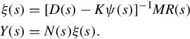
Since M is invertible Eq. (4.84) gives a right polynomial fraction description for the closed-loop transfer function

$\begin{array}{l}\hfill N(s){\widehat{D}}^{-1}(s)=N(s){[M^{-1}D(s)-M^{-1}K\psi (s)]}^{-1}.\end{array}$

This description is not necessarily coprime, though $\widehat{D}(s)$ is column reduced.

Reflection on Eq. (4.85) reveals that choices of K and invertible M provide complete freedom to specify the coefficients of $\widehat{D}(s).$ In detail, suppose

$\begin{array}{l}\hfill D(s)=D_{hc}\Delta (s)+D_l\psi (s)\end{array}$

and suppose the desired $\widehat{D}(s)$ is

$\begin{array}{l}\hfill \widehat{D}(s)={\widehat{D}}_{hc}\Delta (s)+{\widehat{D}}_l\psi (s).\end{array}$

Then the feedback gains

$\begin{array}{l}\hfill M=D_{hc}{\widehat{D}}_{hc}^{-1},K=-M{\widehat{D}}_l+D_l\end{array}$

accomplish the task. Although the choices of K and M do not directly affect N(s), there is an indirect effect in that Eq. (4.85) might not be coprime. This occurs in a more obvious fashion in the single-input, single-output case when linear state feedback places a root of the denominator polynomial coincident with a root of the numerator polynomial.