
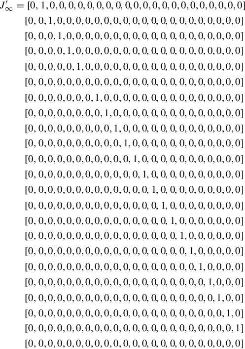
and the infinite Jordan pair (![]() ) (in the sense of Vardulakis [13]) of A(s)
) (in the sense of Vardulakis [13]) of A(s)

It should be noted that the generalized infinite Jordan pair (![]() ), which has dimensions of 4 × 23 and 23 × 23, is much unnecessarily larger than the infinite Jordan pair (
), which has dimensions of 4 × 23 and 23 × 23, is much unnecessarily larger than the infinite Jordan pair (![]() ) with dimensions of only 4 × 5 and 5 × 5. The following matrix
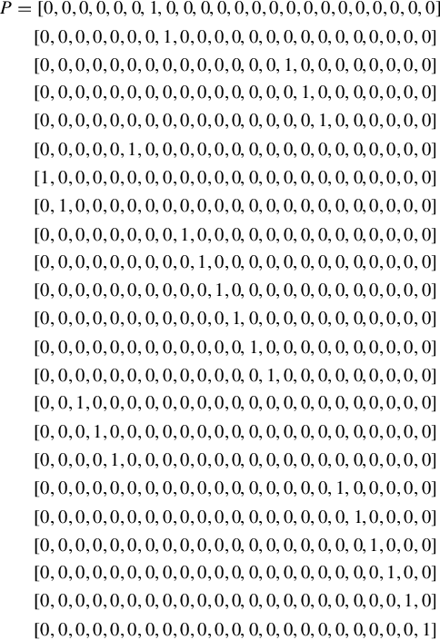
) with dimensions of only 4 × 5 and 5 × 5. The following matrix ![]() is found to delete the redundant information inherited in the generalized infinite Jordan pair.
is found to delete the redundant information inherited in the generalized infinite Jordan pair.
satisfies Theorem 9.2.1. According to Lemma 9.3.2, one has


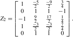
so from
 (9.19)
and from
one obtains
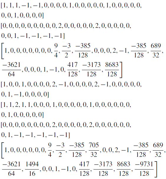
Hence, by Theorem 9.3.1 we have constructed the refined resolvent decomposition for the regular polynomial matrix A(s) as follows

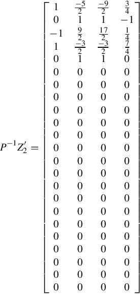
Based on Algorithm 9.4.1, a procedure in the symbolic computational package Maple has been developed and has been implemented to carry out the above calculations. Note that in the above refined resolvent decomposition the matrices ![]() ,
, ![]() , and Z2 have the minimal dimensions of 4 × 5, 5 × 5, and 5 × 4. Compared to the resolvent decomposition of Gohberg et al. [17] given by
, and Z2 have the minimal dimensions of 4 × 5, 5 × 5, and 5 × 4. Compared to the resolvent decomposition of Gohberg et al. [17] given by

where ![]() ,
, ![]() , and
, and ![]() are given by Eqs. (9.17), (9.18), (9.19), respectively, due to the fact that the redundant information has been deleted, the above refined resolvent decomposition is obviously in a much more concise form, which will definitely bring some convenience when applied to the solution of the regular PMDs.
are given by Eqs. (9.17), (9.18), (9.19), respectively, due to the fact that the redundant information has been deleted, the above refined resolvent decomposition is obviously in a much more concise form, which will definitely bring some convenience when applied to the solution of the regular PMDs.
9.5 Conclusions
So far there have been two special resolvent decompositions proposed in the literature through which the solution of a PMD may be expressed. These are based on two different interpretations of the notion of infinite Jordan pair, the first being due to Gohberg et al. [17], and the second due to Vardulakis [13]. The resolvent decomposition proposed by Gohberg et al. [17] uses a certain redundant system structure that results in overly large dimensions of the infinite Jordan pair, though it is relatively simple to calculate the infinite Jordan pair. On the other hand, the approach proposed by Vardulakis [13] uses only the relevant system structure, without using redundant information, and the resulting infinite Jordan pair is of minimal dimensions. It is, however, relatively more difficult to compute the required special realizations.
In this chapter, it is established that the redundant information contained in the infinite Jordan pair defined by Gohberg et al. [17] can be deleted through a certain transformation. Based on this, a natural connection between the infinite Jordan pairs defined by Gohberg et al. [17] and that of Vardulakis [13] has been exploited. This facilitates a refinement of the resolvent decomposition. This resulting resolvent decomposition more precisely reflects the relevant system structure and thereby inherits the advantages of both the decompositions of Gohberg et al. [17] and Vardulakis [13].
In the proposed approach the matrices ![]() in Eq. (9.3) are formulated explicitly, which means this method is constructive. The main idea in this proposed approach is to calculate an elementary matrix P, which is very easy to obtain, to delete the redundant information, then to propose the refined resolvent decomposition. This elementary matrix has the effect of deleting the redundant information in two ways. First, it deletes the redundant information in those blocks in the infinite Jordan pair of Gohberg et al. [17] that correspond to the infinite zeros and bring them into the correct sizes. Second, it deletes the whole blocks in the infinite Jordan pair of Gohberg et al. [17] that correspond to the infinite poles and the whole blocks that are not dynamically important. This elementary matrix serves to transform the partitioned block matrix in
in Eq. (9.3) are formulated explicitly, which means this method is constructive. The main idea in this proposed approach is to calculate an elementary matrix P, which is very easy to obtain, to delete the redundant information, then to propose the refined resolvent decomposition. This elementary matrix has the effect of deleting the redundant information in two ways. First, it deletes the redundant information in those blocks in the infinite Jordan pair of Gohberg et al. [17] that correspond to the infinite zeros and bring them into the correct sizes. Second, it deletes the whole blocks in the infinite Jordan pair of Gohberg et al. [17] that correspond to the infinite poles and the whole blocks that are not dynamically important. This elementary matrix serves to transform the partitioned block matrix in ![]() that corresponds to the redundant information into zero, the resulting refined resolvent decomposition is thus of minimal dimensions. Further, by using this elementary matrix the mechanism of decoupling in the solution of Gohberg et al. [17] is explained clearly. This refined resolvent decomposition facilitates computation of the inverse matrix of A(s) due to the fact that the dimensions of the matrices used are minimal. Once the refined resolvent decomposition is obtained, the generalized infinite Jordan pair and the elementary matrix P are no longer needed in the calculation of the solution of the regular PMD. This therefore presents another merit to this method, which is algorithmically attractive when applied in actual computation.
that corresponds to the redundant information into zero, the resulting refined resolvent decomposition is thus of minimal dimensions. Further, by using this elementary matrix the mechanism of decoupling in the solution of Gohberg et al. [17] is explained clearly. This refined resolvent decomposition facilitates computation of the inverse matrix of A(s) due to the fact that the dimensions of the matrices used are minimal. Once the refined resolvent decomposition is obtained, the generalized infinite Jordan pair and the elementary matrix P are no longer needed in the calculation of the solution of the regular PMD. This therefore presents another merit to this method, which is algorithmically attractive when applied in actual computation.
Based on this refined resolvent decomposition, the complete solution of regular PMDs has then been investigated. This solution presents the zero input response and the zero state response precisely and takes into account the impulsive properties of the system. An algorithm, which has already been implemented in the symbolic computational package Maple, for the investigation of this refined resolvent decomposition is provided.
Compared with the complete solution of regular PMDs given in Chapter 8, where the solution is proposed based on any resolvent decomposition, the resolvent decomposition obtained in this chapter is minimal, the built solution is thus specific to this refined resolvent decomposition.