Search in book...
Toggle Font Controls
Create new playlist

Name your new playlist

Playlist description (optional)
Sign In

Email address

Password

Forgot Password?

or

Continue with Facebook

Continue with Google
Sign Up

Full Name

Email address

Confirm Email Address

Password

or

Continue with Facebook

Continue with Google

Polynomial fraction description

Abstract

The polynomial matrix fraction description is a mathematically efficient and useful representation for a matrix of rational functions. With application to the transfer function of a multiinput, multioutput linear state equation, the polynomial fraction description can inherit the structural features that, for example, permit natural generalization of minimal realization having established for single-input, single-output state equations. The main aim of this chapter is to lay out a basic introduction to the polynomial fraction description, which is a key mathematical component in the current exposition of the generalized linear multivariable control theory. The main components covered by this chapter are right (left) polynomial fractions, column and row degrees, minimal realization, poles and zeros, and state feedback.

Keywords

Right (left) polynomial fraction; Column (row) degree; Minimal realization; Pole and zero; State feedback

This chapter is dedicated to giving a full introduction to polynomial fraction description, which is important to the main theme in the sequel. The complete description of polynomial fraction description can be found in [32, 55]. For polynomial fraction descriptions of time-varying linear systems, one is referred to [56]. For an introduction to coprime factorization, one finds details in [40]. For the expositions of the Smith form for a polynomial matrix and Smith-McMillan form for a rational matrix, one finds the discussions, for example, in [57]. For the polynomial matrix description and structural controllability of the composite system connected by some structural controllable and observable linear time-invariant subsystems in the representations of the irreducible matrix fraction description, recent developments can be found in [58]. For expositions on system poles and zeros, see [59–65]. A recent paper [66] introduces a block decoupling control technique, which is based on the spectral factors of the denominator of the right matrix fraction description in control design and low order controller. Applications of polynomial matrix factorization into resource allocation of optical communication systems are seen from [67]. The paper [68] proposes an alternative option to model a dynamical power system process, which is based on a matrix polynomial form. The model can be obtained naturally writing the high order differential equations of some components (e.g., transmission line models modeled by sequences of RLC PI circuits in power systems) or some of the subsystems that compose the whole system. For other relevant discussions, see also [13, 66, 69–75].

4.1 Introduction

The polynomial fraction description is a mathematically efficient and useful representation of a matrix of rational functions. With application to the transfer function of a multiinput, multioutput linear state equation, polynomial fraction description can inherit the structural features that, for example, permit natural generalization of minimal realization having established single-input, single-output state equations. The main aim of this chapter is to lay out a basic introduction to the polynomial fraction description, which is a key component in the current exposition of the generalized linear multivariable control theory.

We assume throughout this chapter a continuous-time setting, with G(s) a p × m matrix of strictly proper rational functions of s. Then G(s) is realizable by a time-invariant linear state equation. Reinterpretation for discrete time is straightforward by replacement of the Laplace-transform s by a z-transform z.

4.2 Right polynomial fractions

Matrices of real-coefficient polynomials in s, equivalently polynomials in s with coefficients that are real matrices, provide the mathematical foundation for the new transfer function representation.

Definition 4.2.1

A p × r polynomial matrix P(s) is a matrix with entries that are real-coefficient polynomials in s. A square (p = r) polynomial matrix P(s) is called nonsingular if $det P (s)$ $det P (s)$ is a nonzero polynomial, and unimodular if $det P (s)$ $det P (s)$ is a nonzero real number.

The determinant of a square polynomial is a polynomial (a sum of products of the polynomial entries). Thus an alternative characterization is that a square polynomial matrix P(s) is nonsingular if and only if $det P (s_{0}) \neq 0$ $det P (s_{0}) \neq 0$ for all but a finite number of complex numbers s₀. And P(s) is unimodular if and only if $det P (s_{0}) \neq 0$ $det P (s_{0}) \neq 0$ for all complex numbers s₀.

The adjugate-overdeterminant formula shows that if P(s) is square and nonsingular, then P⁻¹(s) exits and (each entry) is a rational function of s. Also P⁻¹(s) is a polynomial matrix if P(s) is unimodular. Sometimes a polynomial is viewed as a rational function with unity denominator. From the reciprocal-determinant relationship between a matrix and its inverse, P⁻¹(s) is unimodular if P(s) is unimodular. Conversely if P(s) and P⁻¹(s) both are polynomial matrices, then both are unimodular.

Definition 4.2.2

A right polynomial fraction description for the p × m strictly proper rational transfer function G(s) is an expression of the form

$\begin{array}{l} G (s) = N (s) D^{- 1} (s), \end{array}$ $\begin{array}{l} G (s) = N (s) D^{- 1} (s), \end{array}$

(4.1)

where N(s) is a p × m polynomial matrix and D(s) is an m × m nonsingular polynomial matrix. A left polynomial fraction description for G(s) is an expression

$\begin{array}{l} G (s) = D_{L}^{- 1} (s) N_{L} (s), \end{array}$ $\begin{array}{l} G (s) = D_{L}^{- 1} (s) N_{L} (s), \end{array}$

(4.2)

where N_L(s) is a p × m polynomial matrix and D_L(s) is a p × p nonsingular polynomial matrix. The degree of a right polynomial fraction description is the degree of the polynomial $det D (s) .$ $det D (s) .$ Similarly the degree of a left polynomial fraction is the degree of $det D_{L} (s) .$ $det D_{L} (s) .$

Of course this definition is familiar if m = p = 1. In the multiinput, multioutput case, a simple device can be used to exhibit so-called elementary polynomial fractions for G(s). Suppose d(s) is a least common multiple of the denominator polynomials of entries of G(s). (In fact, any common multiple of the denominators can be used.) Then

$\begin{array}{l} N_{d} (s) = d (s) G (s) \end{array}$ $\begin{array}{l} N_{d} (s) = d (s) G (s) \end{array}$

is a p × m polynomial matrix, and we can write either a right or left polynomial fraction description

$\begin{array}{l} G (s) = N_{d} (s) {[d (s) I_{m}]}^{- 1} = {[d (s) I_{p}]}^{- 1} N_{d} (s) . \end{array}$ $\begin{array}{l} G (s) = N_{d} (s) {[d (s) I_{m}]}^{- 1} = {[d (s) I_{p}]}^{- 1} N_{d} (s) . \end{array}$

(4.3)

The degrees of the two descriptions are different in general, and it should not be surprising that lower-degree polynomial fraction descriptions typically can be found if some effort is invested.

In the single-input, single-output case, the issue of common factors in the scalar numerator and denominator polynomials of G(s) arises at this point. The utility of the polynomial fraction representation begins to emerge from the corresponding concept in the matrix case.

Definition 4.2.3

An r × r polynomial matrix R(s) is called a right divisor of the p × r polynomial matrix P(s) if there exists a p × r polynomial matrix $\tilde{P} (s)$ $\tilde{P} (s)$ such that

$\begin{array}{l} P (s) = \tilde{P} (s) R (s) . \end{array}$ $\begin{array}{l} P (s) = \tilde{P} (s) R (s) . \end{array}$

If a right divisor R(s) is nonsingular, then P(s)R⁻¹(s) is a p × r polynomial matrix. Also if P(s) is square and nonsingular, then every right divisor of P(s) is nonsingular.

To become accustomed to these notions, it helps to reflect on the case of scalar polynomials. There a right divisor is simply a factor of the polynomial. For polynomial matrices the situation is roughly similar.

Next we consider a matrix-polynomial extension of the concept of a common factor of two scalar polynomials. Since one of the polynomial matrices is always square in our application to transfer function representation, attention is restricted to that situation.

Definition 4.2.4

Suppose P(s) is a p × r polynomial matrix and Q(s) is an r × r polynomial matrix. If the r × r polynomial matrix R(s) is a right divisor of both, then R(s) is called a common right divisor of P(s) and Q(s). We call R(s) a greatest common right divisor of P(s) and Q(s) if it is a common right divisor, and if any other common right divisor of P(s) and Q(s) is a right divisor of R(s). If all common right divisors of P(s) and Q(s) are unimodular, then P(s) and Q(s) are called right coprime.

For polynomial fraction descriptions of a transfer function, one of the polynomial matrices is always nonsingular, so only nonsingular common right divisors occur. Suppose G(s) is given by the right polynomial fraction description

$\begin{array}{l} G (s) = N (s) D^{- 1} (s) \end{array}$ $\begin{array}{l} G (s) = N (s) D^{- 1} (s) \end{array}$

and that R(s) is a common right divisor of N(s) and D(s). Then

$\begin{array}{l} \tilde{N} (s) = N (s) R^{- 1} (s), \tilde{D} (s) = D (s) R^{- 1} (s) \end{array}$ $\begin{array}{l} \tilde{N} (s) = N (s) R^{- 1} (s), \tilde{D} (s) = D (s) R^{- 1} (s) \end{array}$

(4.4)

are polynomial matrices, and they provide another right polynomial fraction description for G(s) since

$\begin{array}{l} \tilde{N} (s) {\tilde{D}}^{- 1} (s) = N (s) R^{- 1} (s) R (s) D^{- 1} (s) = G (s) . \end{array}$ $\begin{array}{l} \tilde{N} (s) {\tilde{D}}^{- 1} (s) = N (s) R^{- 1} (s) R (s) D^{- 1} (s) = G (s) . \end{array}$

The degree of this new polynomial fraction description is no greater than the degree of the original since

$\begin{array}{l} \deg [det D (s)] = \deg [det \tilde{D} (s)] + \deg [det R (s)] . \end{array}$ $\begin{array}{l} \deg [det D (s)] = \deg [det \tilde{D} (s)] + \deg [det R (s)] . \end{array}$

Of course the largest degree reduction occurs if R(s) is a greatest common right divisor, and no reduction occurs if N(s) and D(s) are right coprime. This discussion indicates that exacting common right divisors of a right polynomial fraction is a generalization of the process of canceling common factors in a scalar rational function.

Computation of the greatest common right divisors can be based on the capabilities of elementary row operations on a polynomial matrix-operation similar to the elementary row operations on a matrix of real numbers. To set up this approach we present a preliminary result.

Theorem 4.2.1

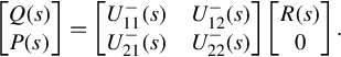
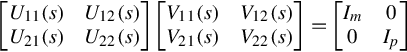
Suppose P(s) is a p × r polynomial matrix and Q(s) is an r × r polynomial matrix. If a unimodular (p + r) × (p + r) polynomial matrix U(s) and an r × r polynomial matrix R(s) are such that

$\begin{array}{l} U (s) [\begin{array}{l} Q (s) \\ P (s) \end{array}] = [\begin{array}{l} R (s) \\ 0 \end{array}] \end{array}$ $\begin{array}{l} U (s) [\begin{array}{l} Q (s) \\ P (s) \end{array}] = [\begin{array}{l} R (s) \\ 0 \end{array}] \end{array}$

si17_e (4.5)

then R(s) is a greatest common right divisor of P(s) and Q(s).

Proof

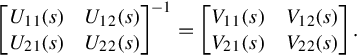
Partition U(s) in the form

$\begin{array}{l} U (s) = [\begin{array}{l} U_{11} (s) & U_{12} (s) \\ U_{21} (s) & U_{22} (s) \end{array}], \end{array}$ $\begin{array}{l} U (s) = [\begin{array}{l} U_{11} (s) & U_{12} (s) \\ U_{21} (s) & U_{22} (s) \end{array}], \end{array}$

si18_e (4.6)

where U₁₁(s) is r × r, and U₂₂(s) is p × p. Then the polynomial matrix U⁻¹(s) can be partitioned similarly as

$\begin{array}{l} U^{- 1} (s) = [\begin{array}{l} U_{11}^{-} (s) & U_{12}^{-} (s) \\ U_{21}^{-} (s) & U_{22}^{-} (s) \end{array}] . \end{array}$ $\begin{array}{l} U^{- 1} (s) = [\begin{array}{l} U_{11}^{-} (s) & U_{12}^{-} (s) \\ U_{21}^{-} (s) & U_{22}^{-} (s) \end{array}] . \end{array}$

si19_e

Using this notation to rewrite Eq. (4.5) gives

$\begin{array}{l} [\begin{array}{l} Q (s) \\ P (s) \end{array}] = [\begin{array}{l} U_{11}^{-} (s) & U_{12}^{-} (s) \\ U_{21}^{-} (s) & U_{22}^{-} (s) \end{array}] [\begin{array}{l} R (s) \\ 0 \end{array}] . \end{array}$ $\begin{array}{l} [\begin{array}{l} Q (s) \\ P (s) \end{array}] = [\begin{array}{l} U_{11}^{-} (s) & U_{12}^{-} (s) \\ U_{21}^{-} (s) & U_{22}^{-} (s) \end{array}] [\begin{array}{l} R (s) \\ 0 \end{array}] . \end{array}$

si20_e

That is,

$\begin{array}{l} Q (s) = U_{11}^{-} (s) R (s), P (s) = U_{21}^{-} (s) R (s) . \end{array}$ $\begin{array}{l} Q (s) = U_{11}^{-} (s) R (s), P (s) = U_{21}^{-} (s) R (s) . \end{array}$

Therefore R(s) is a common right divisor of P(s) and Q(s). But, from Eqs. (4.5), (4.6),

$\begin{array}{l} R (s) = U_{11} (s) Q (s) + U_{12} (s) P (s), \end{array}$ $\begin{array}{l} R (s) = U_{11} (s) Q (s) + U_{12} (s) P (s), \end{array}$

(4.7)

so that if R_a(s) is another common right divisor of P(s) and Q(s), say

$\begin{array}{l} Q (s) = {\tilde{Q}}_{a} (s) R_{a} (s), P (s) = {\tilde{P}}_{a} (s) R_{a} (s), \end{array}$ $\begin{array}{l} Q (s) = {\tilde{Q}}_{a} (s) R_{a} (s), P (s) = {\tilde{P}}_{a} (s) R_{a} (s), \end{array}$

then Eq. (4.7) gives

$\begin{array}{l} R (s) = [U_{11} (s) {\tilde{Q}}_{a} (s) + U_{12} (s) {\tilde{P}}_{a} (s)] R_{a} (s) . \end{array}$ $\begin{array}{l} R (s) = [U_{11} (s) {\tilde{Q}}_{a} (s) + U_{12} (s) {\tilde{P}}_{a} (s)] R_{a} (s) . \end{array}$

This shows R_a(s) also is a right divisor of R(s), and thus R(s) is a greatest common right divisor of P(s) and Q(s).

To calculate the greatest common right divisors using Theorem 4.2.1, we consider three types of elementary row operations on a polynomial matrix. First is the interchange of two rows, and second is the multiplication of a row by a nonzero real number. The third is to add to any row a polynomial multiple of another row. Each of these elementary row operations can be represented by premultiplication by a unimodular matrix, as is easily seen by filling in the following argument.

Interchange of rows i and j≠i correspond to premultiplying by a matrix E_a that has a very simple form. The diagonal entries are unity, except that [E_a]_ii = [E_a]_jj = 0, and the off-diagonal entries are zero, except that [E_a]_ij = [E_a]_ji = 1. Multiplication of the ith-row by a real number α≠0 corresponds to premultiplication by a matrix E_b that is diagonal with all diagonal entries unity, except [E_b]_ii = α. Finally, adding to row i a polynomial p(s) times row j, j≠i, corresponds to premultiplication by a matrix E_c(s) that has unity diagonal entries, with off-diagonal entries zero, except [E_c(s)]_ij = p(s).

It is straightforward to show that the determinants of matrices of the form E_a, E_b, and E_c(s) described above are nonzero real numbers. That is, these matrices are unimodular. Also it is easy to show that the inverse of any of these matrices corresponds to another elementary row operation. The diligent might prove that multiplication of a row by a polynomial is not an elementary row operation in the sense of multiplication by a unimodular matrix, thereby burying a frequent misconception.

It should be clear that a sequence of elementary row operations can be represented as premultiplication by a sequence of these elementary unimodular matrices, and thus as a single unimodular premultiplication. We also want to show the converse—that premultiplication by any unimodular matrix can be represented by a sequence of elementary row operations. Then Theorem 4.2.1 provides a method based on elementary row operations for computing a greatest common right divisor R(s) via Eq. (4.5).

That any unimodular matrix can be written as a product of matrices of the form E_a, E_b, and E_c(s) derives easily from a special form for polynomial matrices. We present this special form for the particular case where the polynomial matrix contains a full-dimension nonsingular partition. This suffices for our application to polynomial fraction descriptions, and also avoids some fussy but trivial issues, such as how to handle identical columns, or all-zero columns. Recall the terminology; that a scalar polynomial is called monic if the coefficient of the highest power of s is unity, that the degree of a polynomial is the highest power of s with nonzero coefficient, and that the degree of the zero polynomial is, by convention, $- \infty .$ $- \infty .$

Theorem 4.2.2

Suppose P(s) is a p × r polynomial matrix and Q(s) is an r × r, nonsingular polynomial matrix. Then elementary row operations can be used to transform

$\begin{array}{l} M (s) = [\begin{array}{l} Q (s) \\ P (s) \end{array}] \end{array}$ $\begin{array}{l} M (s) = [\begin{array}{l} Q (s) \\ P (s) \end{array}] \end{array}$

si26_e (4.8)

into row Hermite form described as follows. For k = 1, …, r, all entries of the kth-column below the k, k-entry are zero, and the k, k-entry is nonzero and monic with higher degree than every entry above it in column k. (If the k, k-entry is unity, then all entries above it are zero.)

Proof

Row Hermite form can be computed by an algorithm that is similar to the row reduction process for constant matrices.

Step (i): In the first column of M(s) use row interchange to bring to the first row a lowest-degree entry among nonzero first-column entries. (By nonsingularity of Q(s), there is a nonzero first-column entry.)

Step (ii): Multiply the first row by a real number so that the first column entry is monic.

Step (iii): For each entry m_i1(s) below the first row in the first column, use polynomial division to write

$\begin{array}{l} m_{i 1} (s) = q_{i} (s) m_{11} (s) + r_{i 1} (s), i = 2, \dots, p + r, \end{array}$ $\begin{array}{l} m_{i 1} (s) = q_{i} (s) m_{11} (s) + r_{i 1} (s), i = 2, \dots, p + r, \end{array}$

(4.9)

where each remainder is such that deg r_i1(s) < deg m₁₁(s). (If m_i1(s) = 0, that is $\deg m_{i 1} (s) = - \infty,$ $\deg m_{i 1} (s) = - \infty,$ we set q_i(s) = r_i1(s) = 0. If deg m_i1(s) = 0, then by Step (i) deg m₁₁(s) = 0. Therefore deg q_i(s) = 0 and $\deg r_{i 1} = - \infty,$ $\deg r_{i 1} = - \infty,$ that is, r_i1(s) = 0.)

Step (iv): For i = 2, …, p + r, add to the ith-row the product of − q_i(s) and the first row. The resulting entries in the first column, below the first row, are r₂₁(s), …, r_{p+r, 1}(s), all of which have degrees less than deg m₁₁(s).

Step (v): Repeat Steps (i) through (iv) until all entries of the first column are zero except the first entry. Since the degrees of the entries below the first entry are lowered by at least one in each iteration, a finite number of operations is required.

Proceed to the second column of M(s) and repeat the above steps while ignoring the first row. This results in a monic, nonzero entry m₂₂(s), with all entries below it zero. If m₁₂(s) does not have lower degree than m₂₂(s), then polynomial division of m₁₂(s) by m₂₂(s) as in Step (iii) and an elementary row operation as in Step (iv) replaces m₁₂(s) by a polynomial of degree less than degm₂₂(s). Next repeat the process for the third column of M(s), while ignoring the first two rows. Continuing yields the claimed form on exhausting the columns of M(s).

To complete the connection between unimodular matrices and elementary row operations, suppose in Theorem 4.2.2 that p = 0, and Q(s) is unimodular. Of course the resulting row Hermite form is upper triangular. The diagonal entries must be unity, for a diagonal entry of positive degree would yield a determinant of positive degree, contradicting unimodularity. But then entries above the diagonal must have degree $- \infty .$ $- \infty .$ Thus row Hermite form for a unimodular matrix is the identity matrix. In other words for a unimodular polynomial matrix U(s) there is a sequence of elementary row operations, say E_a, E_b, E_c(s), …, E_b, such that

$\begin{array}{l} [E_{a} E_{b} E_{c} (s) \dots E_{b}] U (s) = I . \end{array}$ $\begin{array}{l} [E_{a} E_{b} E_{c} (s) \dots E_{b}] U (s) = I . \end{array}$

(4.10)

This obviously gives U(s) as the sequence of elementary row operations on the identity specified by

$\begin{array}{l} U (s) = [E_{b}^{- 1} \dots E_{c}^{- 1} (s) E_{b}^{- 1} E_{a}^{- 1}] I \end{array}$ $\begin{array}{l} U (s) = [E_{b}^{- 1} \dots E_{c}^{- 1} (s) E_{b}^{- 1} E_{a}^{- 1}] I \end{array}$

and premultiplication of a matrix by U(s) thus corresponds to application of a sequence of elementary row operations. Therefore Theorem 4.2.1 can be restated, for the case of nonsingular Q(s), in terms of elementary row operations rather than premultiplication by a unimodular U(s). If reduction to row Hermite form is used in implementing Eq. (4.5), then the greatest common right divisor R(s) will be an upper-triangular polynomial matrix. Furthermore, if P(s) and Q(s) are right coprime, then Theorem 4.2.2 shows that there is a unimodular U(s) such that Eq. (4.5) is satisfied for R(s) = I_r.

Two different characterizations of right coprimeness are used in the sequel. One is in the form of a polynomial matrix equation, while the other involves rank properties of a complex matrix obtained by evaluation of a polynomial matrix at complex values of s.

Theorem 4.2.3

For a p × r polynomial matrix P(s) and a nonsingular r × r polynomial matrix Q(s), the following statements are equivalent:

(i) The polynomial matrices P(s) and Q(s) are right coprime.

(ii) There exist an r × p polynomial matrix X(s) and an r × r polynomial matrix Y (s) satisfying the so-called Bezout identity

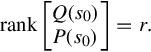
$\begin{array}{l} X (s) P (s) + Y (s) Q (s) = I_{r} . \end{array}$ $\begin{array}{l} X (s) P (s) + Y (s) Q (s) = I_{r} . \end{array}$

(4.11)

(iii) For every complex number s₀,

$\begin{array}{l} rank [\begin{array}{l} Q (s_{0}) \\ P (s_{0}) \end{array}] = r . \end{array}$ $\begin{array}{l} rank [\begin{array}{l} Q (s_{0}) \\ P (s_{0}) \end{array}] = r . \end{array}$

si34_e (4.12)

Proof

Beginning a demonstration that each claim implies the next, first we show that (i) implies (ii). If P(s) and Q(s) are right coprime, then reduction to row Hermite form as in Eq. (4.5) yields polynomial matrices U₁₁(s) and U₁₂(s) such that

$\begin{array}{l} U_{11} (s) Q (s) + U_{12} (s) P (s) = I_{r} \end{array}$ $\begin{array}{l} U_{11} (s) Q (s) + U_{12} (s) P (s) = I_{r} \end{array}$

and this has the form of Eq. (4.11).

To prove that (ii) implies (iii), write the condition (4.11) in the matrix form

$\begin{array}{l} [Y (s) X (s)] [\begin{array}{l} Q (s) \\ P (s) \end{array}] = I_{r} . \end{array}$ $\begin{array}{l} [Y (s) X (s)] [\begin{array}{l} Q (s) \\ P (s) \end{array}] = I_{r} . \end{array}$

si36_e

If s₀ is a complex number for which

$\begin{array}{l} rank [\begin{array}{l} Q (s_{0}) \\ P (s_{0}) \end{array}] < r, \end{array}$ $\begin{array}{l} rank [\begin{array}{l} Q (s_{0}) \\ P (s_{0}) \end{array}] < r, \end{array}$

si37_e

then we have a rank contradiction.

To show (iii) implies (i), suppose that Eq. (4.12) holds and R(s) is a common right divisor of P(s) and Q(s). Then for some p × r polynomial matrix $\tilde{P} (s)$ $\tilde{P} (s)$ and some r × r polynomial matrix $\tilde{Q} (s)$ $\tilde{Q} (s)$

$\begin{array}{l} [\begin{array}{l} Q (s) \\ P (s) \end{array}] = [\begin{array}{l} \tilde{Q} (s) \\ \tilde{P} (s) \end{array}] R (s) . \end{array}$ $\begin{array}{l} [\begin{array}{l} Q (s) \\ P (s) \end{array}] = [\begin{array}{l} \tilde{Q} (s) \\ \tilde{P} (s) \end{array}] R (s) . \end{array}$

si40_e (4.13)

If $det R (s)$ $det R (s)$ is a polynomial of degree at least one and s₀ is a root of this polynomial, then R(s₀) is a complex matrix of less than full rank. Thus we obtain the contradiction

$\begin{array}{l} rank [\begin{array}{l} Q (s_{0}) \\ P (s_{0}) \end{array}] \leq rank R (s_{0}) < r . \end{array}$ $\begin{array}{l} rank [\begin{array}{l} Q (s_{0}) \\ P (s_{0}) \end{array}] \leq rank R (s_{0}) < r . \end{array}$

si42_e

Therefore $det R (s)$ $det R (s)$ is a nonzero constant, that is, R(s) is unimodular. This proves that P(s) and Q(s) are right coprime.

A right polynomial fraction description with N(s) and D(s) right coprime is called simply a coprime right polynomial fraction description. The next result shows that in an important sense all coprime right polynomial fraction descriptions of a given transfer function are equivalent. In particular they all have the same degree.

Theorem 4.2.4

For any two coprime right polynomial fraction descriptions of a strictly proper rational transfer function

$\begin{array}{l} G (s) = N (s) D^{- 1} (s) = N_{a} (s) D_{a}^{- 1} (s), \end{array}$ $\begin{array}{l} G (s) = N (s) D^{- 1} (s) = N_{a} (s) D_{a}^{- 1} (s), \end{array}$

there exists a unimodular polynomial matrix U(s) such that

$\begin{array}{l} N (s) = N_{a} (s) U (s), D (s) = D_{a} (s) U (s) . \end{array}$ $\begin{array}{l} N (s) = N_{a} (s) U (s), D (s) = D_{a} (s) U (s) . \end{array}$

Proof

By Theorem 4.2.3 there exist polynomial matrices X(s), Y (s), A(s), and B(s) such that

$\begin{array}{l} X (s) N_{a} (s) + Y (s) D_{a} (s) = I_{m} \end{array}$ $\begin{array}{l} X (s) N_{a} (s) + Y (s) D_{a} (s) = I_{m} \end{array}$

(4.14)

and

$\begin{array}{l} A (s) N (s) + B (s) D (s) = I_{m} . \end{array}$ $\begin{array}{l} A (s) N (s) + B (s) D (s) = I_{m} . \end{array}$

(4.15)

Since $N (s) D^{- 1} (s) = N_{a} (s) D_{a}^{- 1} (s)$ $N (s) D^{- 1} (s) = N_{a} (s) D_{a}^{- 1} (s)$ , we have N_a(s) = N(s)D⁻¹(s)D_a(s). Substituting this into Eq. (4.14) gives

$\begin{array}{l} X (s) N (s) D^{- 1} (s) D_{a} (s) + Y (s) D_{a} (s) = I_{m} \end{array}$ $\begin{array}{l} X (s) N (s) D^{- 1} (s) D_{a} (s) + Y (s) D_{a} (s) = I_{m} \end{array}$

$\begin{array}{l} X (s) N (s) + Y (s) D (s) = D_{a}^{- 1} (s) D (s) . \end{array}$ $\begin{array}{l} X (s) N (s) + Y (s) D (s) = D_{a}^{- 1} (s) D (s) . \end{array}$

A similar calculation using $N (s) = N_{a} (s) D_{a}^{- 1} (s) D (s)$ $N (s) = N_{a} (s) D_{a}^{- 1} (s) D (s)$ in Eq. (4.15) gives

$\begin{array}{l} A (s) N_{a} (s) + B (s) D_{a} (s) = D^{- 1} (s) D_{a} (s) . \end{array}$ $\begin{array}{l} A (s) N_{a} (s) + B (s) D_{a} (s) = D^{- 1} (s) D_{a} (s) . \end{array}$

Therefore both $D_{a}^{- 1} (s) D (s)$ $D_{a}^{- 1} (s) D (s)$ and D⁻¹(s)D_a(s) are polynomial matrices, and since they are inverses of each other both must be unimodular. Let

$\begin{array}{l} U (s) = D_{a}^{- 1} (s) D (s) . \end{array}$ $\begin{array}{l} U (s) = D_{a}^{- 1} (s) D (s) . \end{array}$

Then

$\begin{array}{l} N (s) = N_{a} (s) U (s), D (s) = D_{a} (s) D_{a}^{- 1} (s) D (s) = D_{a} (s) U (s) \end{array}$ $\begin{array}{l} N (s) = N_{a} (s) U (s), D (s) = D_{a} (s) D_{a}^{- 1} (s) D (s) = D_{a} (s) U (s) \end{array}$

and the proof is complete.

4.3 Left polynomial fraction

Before going further we pause to consider left polynomial fraction descriptions and their relation to right polynomial fraction descriptions of the same transfer function. This means repeating much of the right-handed development, and proofs of the results are left as unlisted exercises.

Definition 4.3.1

A q × q polynomial matrix L(s) is called a left divisor of the q × p polynomial matrix P(s) if there exists a q × p polynomial matrix $\tilde{P} (s)$ $\tilde{P} (s)$ such that

$\begin{array}{l} P (s) = L (s) \tilde{P} (s) . \end{array}$ $\begin{array}{l} P (s) = L (s) \tilde{P} (s) . \end{array}$

(4.16)

Definition 4.3.2

If P(s) is a q × p polynomial matrix and Q(s) is a q × q polynomial matrix, then a q × q polynomial matrix L(s) is called a common left divisor of P(s) and Q(s) if L(s) is a left divisor of both P(s) and Q(s). We call L(s) a greatest common left divisor of P(s) and Q(s) if it is a common left divisor, and if any other common left divisor of P(s) and Q(s) is a left divisor of L(s). If all common left divisors of P(s) and Q(s) are unimodular, then P(s) and Q(s) are called left coprime.

Theorem 4.3.1

Suppose P(s) is a q × p polynomial matrix and Q(s) is a q × q polynomial matrix. If a (q + p) × (q + p) unimodular polynomial matrix U(s) and a q × q polynomial matrix L(s) are such that

$\begin{array}{l} [Q (s) P (s)] U (s) = [L (s) 0], \end{array}$ $\begin{array}{l} [Q (s) P (s)] U (s) = [L (s) 0], \end{array}$

(4.17)

then L(s) is a greatest common left divisor of P(s) and Q(s).

Three types of elementary column operations can be represented by postmultiplication by a unimodular matrix. The first is interchange of two columns, and the second is multiplication of any column by a nonzero real number. The third elementary column operation is addition to any column of a polynomial multiple of another column. It is easy to check that a sequence of these elementary column operations can be represented by postmultiplication by a unimodular matrix. That postmultiplication by any unimodular matrix can be represented by an appropriate sequence of elementary column operations is a consequence of another special form, introduced below for the class of polynomial matrices of interest.

Theorem 4.3.2

Suppose P(s) is a q × p polynomial matrix and Q(s) is a q × q nonsingular polynomial matrix. Then elementary column operations can be used to transform

$\begin{array}{l} M (s) = [Q (s) P (s)] \end{array}$ $\begin{array}{l} M (s) = [Q (s) P (s)] \end{array}$

into a column Hermite form described as follows. For k = 1, …, q, all entries of the kth-row to the right of the k, k-entry are zero, and the k, k-entry is monic with higher degree than any entry to its left. (If the k, k-entry is unity, all entries to its left are zero.)

Theorems 4.3.1 and 4.3.2 together provide a method for computing greatest common left divisors using elementary column operations to obtain column Hermite form. The polynomial matrix L(s) in Eq. (4.17) will be lower-triangular.

Theorem 4.3.3

For a q × p polynomial matrix P(s) and a nonsingular q × q polynomial matrix Q(s), the following statements are equivalent:

(i) The polynomial matrices P(s) and Q(s) are left coprime.

(ii) There exist a p × q polynomial matrix X(s) and a q × q polynomial matrix Y (s) such that

$\begin{array}{l} P (s) X (s) + Q (s) Y (s) = I_{q} . \end{array}$ $\begin{array}{l} P (s) X (s) + Q (s) Y (s) = I_{q} . \end{array}$

(4.18)

(iii) For every complex number s₀,

$\begin{array}{l} rank [Q (s_{0}) P (s_{0})] = q . \end{array}$ $\begin{array}{l} rank [Q (s_{0}) P (s_{0})] = q . \end{array}$

(4.19)

Naturally a left polynomial fraction description composed of left coprime polynomial matrices is called a coprime left polynomial fraction description.

Theorem 4.3.4

For any two coprime left polynomial fraction descriptions of a strictly proper rational transfer function

$\begin{array}{l} G (s) = D^{- 1} (s) N (s) = D_{a}^{- 1} (s) N_{a} (s), \end{array}$ $\begin{array}{l} G (s) = D^{- 1} (s) N (s) = D_{a}^{- 1} (s) N_{a} (s), \end{array}$

there exists a unimodular polynomial matrix U(s) such that

$\begin{array}{l} N (s) = U (s) N_{a} (s), D (s) = U (s) D_{a} (s) . \end{array}$ $\begin{array}{l} N (s) = U (s) N_{a} (s), D (s) = U (s) D_{a} (s) . \end{array}$

Suppose that we begin with the elementary right polynomial fraction description and the elementary left polynomial fraction description in Eq. (4.3) for a given strictly proper rational transfer function G(s). Then appropriate greatest common divisors can be extracted to obtain a coprime right polynomial fraction description, and a coprime left polynomial fraction description for G(s). We now show that these two coprime polynomial fraction descriptions have the same degree. An economical demonstration relies on a particular polynomial-matrix inversion formula.

Lemma 4.3.1

Suppose that V₁₁(s) is a m × m nonsingular polynomial matrix and

$\begin{array}{l} V (s) = [\begin{array}{l} V_{11} (s) & V_{12} (s) \\ V_{21} (s) & V_{22} (s) \end{array}], \end{array}$ $\begin{array}{l} V (s) = [\begin{array}{l} V_{11} (s) & V_{12} (s) \\ V_{21} (s) & V_{22} (s) \end{array}], \end{array}$

si64_e (4.20)

is an (m + p) × (m + p) nonsingular polynomial matrix. Then defining the matrix of rational functions $V_{a} (s) = V_{22} (s) - V_{21} (s) V_{11}^{- 1} (s) V_{12} (s)$ $V_{a} (s) = V_{22} (s) - V_{21} (s) V_{11}^{- 1} (s) V_{12} (s)$

(i) $det V (s) = det [V_{11} (s)] \cdot det [V_{a} (s)],$ $det V (s) = det [V_{11} (s)] \cdot det [V_{a} (s)],$

(ii) $det V_{a} (s)$ $det V_{a} (s)$ is a nonzero rational function,

(iii) the inverse of V (s) is

$\begin{array}{l} V^{- 1} (s) = [\begin{array}{l} V_{11}^{- 1} (s) + V_{11}^{- 1} (s) V_{12} (s) V_{a}^{- 1} (s) V_{21} (s) V_{11}^{- 1} (s) & - V_{11}^{- 1} (s) V_{12} (s) V_{a}^{- 1} (s) \\ - V_{a}^{- 1} (s) V_{21} (s) V_{11}^{- 1} (s) & V_{a}^{- 1} (s) . \end{array}] \end{array}$ $\begin{array}{l} V^{- 1} (s) = [\begin{array}{l} V_{11}^{- 1} (s) + V_{11}^{- 1} (s) V_{12} (s) V_{a}^{- 1} (s) V_{21} (s) V_{11}^{- 1} (s) & - V_{11}^{- 1} (s) V_{12} (s) V_{a}^{- 1} (s) \\ - V_{a}^{- 1} (s) V_{21} (s) V_{11}^{- 1} (s) & V_{a}^{- 1} (s) . \end{array}] \end{array}$

si68_e

Proof

A partitioned calculation verifies

$\begin{array}{l} [\begin{array}{l} I_{m} & 0_{m \times p} \\ - V_{21} (s) V_{11}^{- 1} (s) & I_{p} \end{array}] V (s) = [\begin{array}{l} V_{11} (s) & V_{12} (s) \\ 0 & V_{a} (s) \end{array}] . \end{array}$ $\begin{array}{l} [\begin{array}{l} I_{m} & 0_{m \times p} \\ - V_{21} (s) V_{11}^{- 1} (s) & I_{p} \end{array}] V (s) = [\begin{array}{l} V_{11} (s) & V_{12} (s) \\ 0 & V_{a} (s) \end{array}] . \end{array}$

si69_e (4.21)

Using the obvious determinant identity for block-triangular matrices, in particular

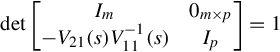
$\begin{array}{l} det [\begin{array}{l} I_{m} & 0_{m \times p} \\ - V_{21} (s) V_{11}^{- 1} (s) & I_{p} \end{array}] = 1 \end{array}$ $\begin{array}{l} det [\begin{array}{l} I_{m} & 0_{m \times p} \\ - V_{21} (s) V_{11}^{- 1} (s) & I_{p} \end{array}] = 1 \end{array}$

si70_e

gives

$\begin{array}{l} det V (s) = det [V_{11} (s)] \cdot det [V_{a} (s)] . \end{array}$ $\begin{array}{l} det V (s) = det [V_{11} (s)] \cdot det [V_{a} (s)] . \end{array}$

Since V (s) and V₁₁(s) are nonsingular polynomial matrices, this proves that $det V_{a} (s)$ $det V_{a} (s)$ is a nonzero rational function, that is, $V_{a}^{- 1} (s)$ $V_{a}^{- 1} (s)$ exists. To establish (iii), multiply Eq. (4.21) on the left by

$\begin{array}{l} [\begin{array}{l} V_{11}^{- 1} (s) & 0 \\ 0 & V_{a}^{- 1} (s) \end{array}] [\begin{array}{l} I_{m} & - V_{12} (s) V_{a}^{- 1} (s) \\ 0 & I_{p} \end{array}] \end{array}$ $\begin{array}{l} [\begin{array}{l} V_{11}^{- 1} (s) & 0 \\ 0 & V_{a}^{- 1} (s) \end{array}] [\begin{array}{l} I_{m} & - V_{12} (s) V_{a}^{- 1} (s) \\ 0 & I_{p} \end{array}] \end{array}$

si74_e

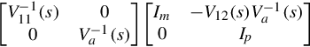
to obtain

$\begin{array}{l} [\begin{array}{l} V_{11}^{- 1} (s) + V_{11}^{- 1} (s) V_{12} (s) V_{a}^{- 1} (s) V_{21} (s) V_{11}^{- 1} (s) & - V_{11}^{- 1} (s) V_{12} (s) V_{a}^{- 1} (s) \\ - V_{a}^{- 1} (s) V_{21} (s) V_{11}^{- 1} (s) & V_{a}^{- 1} (s) \end{array}] \\ V (s) = [\begin{array}{l} I_{m} & 0 \\ 0 & I_{p} \end{array}] \end{array}$ $\begin{array}{l} [\begin{array}{l} V_{11}^{- 1} (s) + V_{11}^{- 1} (s) V_{12} (s) V_{a}^{- 1} (s) V_{21} (s) V_{11}^{- 1} (s) & - V_{11}^{- 1} (s) V_{12} (s) V_{a}^{- 1} (s) \\ - V_{a}^{- 1} (s) V_{21} (s) V_{11}^{- 1} (s) & V_{a}^{- 1} (s) \end{array}] \\ V (s) = [\begin{array}{l} I_{m} & 0 \\ 0 & I_{p} \end{array}] \end{array}$

si75_e

and the proof is complete.

Theorem 4.3.5

Suppose that a strictly proper rational transfer function is represented by a coprime right polynomial fraction and a coprime left polynomial fraction

$\begin{array}{l} G (s) = N (s) D^{- 1} (s) = D_{L}^{- 1} (s) N_{L} (s) . \end{array}$ $\begin{array}{l} G (s) = N (s) D^{- 1} (s) = D_{L}^{- 1} (s) N_{L} (s) . \end{array}$

(4.22)

Then there exists a nonzero constant α such that $det D (s) = α det D_{L} (s) .$ $det D (s) = α det D_{L} (s) .$

Proof

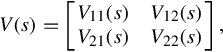
By right-coprimeness of N(s) and D(s) there exists an (m + p) × (m + p) unimodular polynomial matrix

$\begin{array}{l} U (s) = [\begin{array}{l} U_{11} (s) & U_{12} (s) \\ U_{21} (s) & U_{22} (s) \end{array}] \end{array}$ $\begin{array}{l} U (s) = [\begin{array}{l} U_{11} (s) & U_{12} (s) \\ U_{21} (s) & U_{22} (s) \end{array}] \end{array}$

si78_e

such that

$\begin{array}{l} [\begin{array}{l} U_{11} (s) & U_{12} (s) \\ U_{21} (s) & U_{22} (s) \end{array}] [\begin{array}{l} D (s) \\ N (s) \end{array}] = [\begin{array}{l} I_{m} \\ 0 \end{array}] . \end{array}$ $\begin{array}{l} [\begin{array}{l} U_{11} (s) & U_{12} (s) \\ U_{21} (s) & U_{22} (s) \end{array}] [\begin{array}{l} D (s) \\ N (s) \end{array}] = [\begin{array}{l} I_{m} \\ 0 \end{array}] . \end{array}$

si79_e (4.23)

For notational convenience let

$\begin{array}{l} {[\begin{array}{l} U_{11} (s) & U_{12} (s) \\ U_{21} (s) & U_{22} (s) \end{array}]}^{- 1} = [\begin{array}{l} V_{11} (s) & V_{12} (s) \\ V_{21} (s) & V_{22} (s) \end{array}] . \end{array}$ $\begin{array}{l} {[\begin{array}{l} U_{11} (s) & U_{12} (s) \\ U_{21} (s) & U_{22} (s) \end{array}]}^{- 1} = [\begin{array}{l} V_{11} (s) & V_{12} (s) \\ V_{21} (s) & V_{22} (s) \end{array}] . \end{array}$

si80_e

Each V_ij(s) is a polynomial matrix, and in particular Eq. (4.23) gives

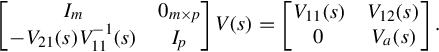
$\begin{array}{l} V_{11} (s) = D (s), V_{21} (s) = N (s) . \end{array}$ $\begin{array}{l} V_{11} (s) = D (s), V_{21} (s) = N (s) . \end{array}$

Therefore V₁₁(s) is nonsingular, and calling on Lemma 4.3.1 we have that

$\begin{array}{l} U_{22} (s) = {[V_{22} (s) - V_{21} (s) V_{11}^{- 1} (s) V_{12} (s)]}^{- 1}, \end{array}$ $\begin{array}{l} U_{22} (s) = {[V_{22} (s) - V_{21} (s) V_{11}^{- 1} (s) V_{12} (s)]}^{- 1}, \end{array}$

which of course is a polynomial matrix, is nonsingular. Furthermore writing

$\begin{array}{l} [\begin{array}{l} U_{11} (s) & U_{12} (s) \\ U_{21} (s) & U_{22} (s) \end{array}] [\begin{array}{l} V_{11} (s) & V_{12} (s) \\ V_{21} (s) & V_{22} (s) \end{array}] = [\begin{array}{l} I_{m} & 0 \\ 0 & I_{p} \end{array}] \end{array}$ $\begin{array}{l} [\begin{array}{l} U_{11} (s) & U_{12} (s) \\ U_{21} (s) & U_{22} (s) \end{array}] [\begin{array}{l} V_{11} (s) & V_{12} (s) \\ V_{21} (s) & V_{22} (s) \end{array}] = [\begin{array}{l} I_{m} & 0 \\ 0 & I_{p} \end{array}] \end{array}$

si83_e (4.24)

gives, in the 2,2-block,

$\begin{array}{l} U_{21} (s) V_{12} (s) + U_{22} (s) V_{22} (s) = I_{p} . \end{array}$ $\begin{array}{l} U_{21} (s) V_{12} (s) + U_{22} (s) V_{22} (s) = I_{p} . \end{array}$

By Theorem 4.3.3 this implies that U₂₁(s) and U₂₂(s) are left coprime. Also, from the 2,1-block,

$\begin{array}{l} U_{21} (s) V_{11} (s) + U_{22} (s) V_{21} (s) = U_{21} (s) D (s) + U_{22} (s) N (s) = 0 . \end{array}$ $\begin{array}{l} U_{21} (s) V_{11} (s) + U_{22} (s) V_{21} (s) = U_{21} (s) D (s) + U_{22} (s) N (s) = 0 . \end{array}$

(4.25)

Thus we can write, from Eq. (4.25)

$\begin{array}{l} G (s) = N (s) D^{- 1} (s) = - U_{22}^{- 1} (s) U_{21} (s) . \end{array}$ $\begin{array}{l} G (s) = N (s) D^{- 1} (s) = - U_{22}^{- 1} (s) U_{21} (s) . \end{array}$

(4.26)

This is a coprime left polynomial fraction description for G(s). Again using Lemma 4.3.1, and the unimodularity of V (s), there exists a nonzero constant α such that

$\begin{array}{l} \begin{matrix} det [\begin{array}{l} V_{11} (s) & V_{12} (s) \\ V_{21} (s) & V_{22} (s) \end{array}] & = det [V_{11} (s)] \cdot det [V_{22} (s) - V_{21} (s) V_{11}^{- 1} (s) V_{12} (s)] \\ = det [D (s)] \cdot det [U_{22}^{- 1} (s)] \\ = \frac{det D (s)}{det U_{22} (s)} = \frac{1}{α} . \end{matrix} \end{array}$ $\begin{array}{l} \begin{matrix} det [\begin{array}{l} V_{11} (s) & V_{12} (s) \\ V_{21} (s) & V_{22} (s) \end{array}] & = det [V_{11} (s)] \cdot det [V_{22} (s) - V_{21} (s) V_{11}^{- 1} (s) V_{12} (s)] \\ = det [D (s)] \cdot det [U_{22}^{- 1} (s)] \\ = \frac{det D (s)}{det U_{22} (s)} = \frac{1}{α} . \end{matrix} \end{array}$

si87_e (4.27)

Therefore, for the coprime left polynomial fraction description in Eq. (4.26), we have $det U_{22} (s) = α det D (s) .$ $det U_{22} (s) = α det D (s) .$ Finally, using the unimodular relation between coprime left polynomial fractions in Theorem 4.3.4, such a determinant formula, with possibly a different nonzero constant, must hold for any coprime left polynomial fraction description for G(s).

4.4 Column and row degrees

There is an additional technical consideration that complicates the representation of a strictly proper rational transfer function by polynomial fraction descriptions. First, we introduce terminology for matrix polynomials that is related to the notion of the degree of a scalar polynomial. Recall again conventions that the degree of a nonzero constant is zero, and the degree of the polynomial 0 is $- \infty .$ $- \infty .$

Definition 4.4.1

For a p × r polynomial matrix P(s), the degree of the highest-degree polynomial in the jth-column of P(s), written c_j[P], is called the jth-column degree of P(s). The column degree coefficient matrix for P(s), written P_hc, is the real p × r matrix with i, j-entry given by the coefficient of $s^{c_{j} [P]}$ $s^{c_{j} [P]}$ in the i, j-entry of P(s). If P(s) is square and nonsingular, then it is called column reduced if

$\begin{array}{l} \deg [det P (s)] = c_{1} [P] + \dots + c_{p} [P] . \end{array}$ $\begin{array}{l} \deg [det P (s)] = c_{1} [P] + \dots + c_{p} [P] . \end{array}$

(4.28)

If P(s) is square, then the Laplace expansion of the determinant about columns shows that the degree of $det P (s)$ $det P (s)$ cannot be greater than c₁[P] + ⋯ + c_p[P]. But it can be less.

The issue that requires attention involves the column degrees of D(s) in a right polynomial fraction description for a strictly proper rational transfer function. It is clear in the m = p = 1 case that this column degree plays an important role in realization considerations, for example. The same is true in the multiinput, multioutput case, and the complication is that column degrees of D(s) can be artificially high, and they can change in the process of postmultiplication by a unimodular matrix. Therefore two coprime right polynomial fraction descriptions for G(s), as in Theorem 4.2.4, can be such that D(s) and D_a(s) have different column degrees, even though the degrees of the polynomials $det D (s)$ $det D (s)$ and $det D_{a} (s)$ $det D_{a} (s)$ are the same.

The first step in investigating this situation is to characterize column-reduced polynomial matrices in a way that does not involve computing a determinant. Using Definition 4.4.1 it is convenient to write a p × p polynomial matrix P(s) in the form

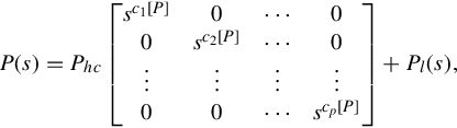
$\begin{array}{l} P (s) = P_{h c} [\begin{array}{l} s^{c_{1} [P]} & 0 & \dots & 0 \\ 0 & s^{c_{2} [P]} & \dots & 0 \\ ⋮ & ⋮ & ⋮ & ⋮ \\ 0 & 0 & \dots & s^{c_{p} [P]} \end{array}] + P_{l} (s), \end{array}$ $\begin{array}{l} P (s) = P_{h c} [\begin{array}{l} s^{c_{1} [P]} & 0 & \dots & 0 \\ 0 & s^{c_{2} [P]} & \dots & 0 \\ ⋮ & ⋮ & ⋮ & ⋮ \\ 0 & 0 & \dots & s^{c_{p} [P]} \end{array}] + P_{l} (s), \end{array}$

si95_e (4.29)

where P_l(s) is a p × p polynomial matrix in which each entry of the jth-column has degree strictly less than c_j[P]. (We use this notation only when P(s) is nonsingular, so that c₁[P], …, c_p[P] ≥ 0.)

Theorem 4.4.1

If P(s) is a p × p nonsingular polynomial matrix, then P(s) is column reduced if and only if P_hc is invertible.

Proof

We can write, using the representation (4.29)

$\begin{array}{l} s^{- c_{1} [P] - \dots - c_{p} [P]} \cdot det P (s) & = det [P (s) \cdot d i a g o n a l {s^{- c_{1} [P]}, \dots, s^{- c_{p} [P]}}] \\ = det [P_{h c} + P_{l} (s) \cdot d i a g o n a l {s^{- c_{1} [P]}, \dots, s^{- c_{p} [P]}}] \\ = det [P_{h c} + \tilde{P} (s^{- 1})], \end{array}$ $\begin{array}{l} s^{- c_{1} [P] - \dots - c_{p} [P]} \cdot det P (s) & = det [P (s) \cdot d i a g o n a l {s^{- c_{1} [P]}, \dots, s^{- c_{p} [P]}}] \\ = det [P_{h c} + P_{l} (s) \cdot d i a g o n a l {s^{- c_{1} [P]}, \dots, s^{- c_{p} [P]}}] \\ = det [P_{h c} + \tilde{P} (s^{- 1})], \end{array}$

si96_e (4.30)

where $\tilde{P} (s^{- 1})$ $\tilde{P} (s^{- 1})$ is a matrix with entries that are polynomials in s⁻¹ that have no constant terms, that is, no s⁰ terms. A key fact in the remaining argument is that, viewing s as real and positive, letting $s \to \infty$ $s \to \infty$ yields $\tilde{P} (s^{- 1}) \to 0 .$ $\tilde{P} (s^{- 1}) \to 0 .$ Also the determinant of a matrix is a continuous function of the matrix entries, so limit and determinant can be interchanged. In particular we can write

$\begin{array}{l} \begin{matrix} lim_{s \to \infty} [s^{- c_{1} [P] - \dots - c_{p} [P]} \cdot det P (s)] & = lim_{s \to \infty} det [P_{h c} + \tilde{P} (s^{- 1})] \\ = det {lim_{s \to \infty} [P_{h c} + \tilde{P} (s^{- 1})]} \\ = det P_{h c} . \end{matrix} \end{array}$ $\begin{array}{l} \begin{matrix} lim_{s \to \infty} [s^{- c_{1} [P] - \dots - c_{p} [P]} \cdot det P (s)] & = lim_{s \to \infty} det [P_{h c} + \tilde{P} (s^{- 1})] \\ = det {lim_{s \to \infty} [P_{h c} + \tilde{P} (s^{- 1})]} \\ = det P_{h c} . \end{matrix} \end{array}$

si100_e (4.31)

Using Eq. (4.28) the left side of Eq. (4.31) is a nonzero constant if and only if P(s) is column reduced, and thus the proof is complete.

Consider a coprime right polynomial fraction description N(s)D⁻¹(s), where D(s) is not column reduced. We next show that elementary column operations on D(s) (postmultiplication by a unimodular matrix U(s)) can be used to reduce individual column degrees, and thus compute a new coprime right polynomial fraction description

$\begin{array}{l} \tilde{N} (s) = N (s) U (s), \tilde{D} (s) = D (s) U (s), \end{array}$ $\begin{array}{l} \tilde{N} (s) = N (s) U (s), \tilde{D} (s) = D (s) U (s), \end{array}$

(4.32)

where $\tilde{D} (s)$ $\tilde{D} (s)$ is column reduced. Of course U(s) need not be constructed, explicitly simply perform the same sequence of elementary column operations on N(s) as on D(s) to obtain $\tilde{N} (s)$ $\tilde{N} (s)$ along with $\tilde{D} (s) .$ $\tilde{D} (s) .$

To describe the required calculations, suppose the column degrees of the m × m polynomial matrix D(s) satisfy c₁[D] ≥ c₂[D], …, c_m[D], as can achieved by column interchanges. Using the notation

$\begin{array}{l} D (s) = D_{h c} Δ (s) + D_{l} (s), \end{array}$ $\begin{array}{l} D (s) = D_{h c} Δ (s) + D_{l} (s), \end{array}$

(4.33)

there exists a nonzero m × 1 vector z such that D_hcz = 0, since D(s) is not column reduced. Suppose that the first nonzero entry in z is z_k, and define a corresponding polynomial vector by

$\begin{array}{l} z = [\begin{array}{l} 0 \\ ⋮ \\ 0 \\ z_{k} \\ z_{k + 1} \\ ⋮ \\ z_{m} \end{array}] \to z (s) = [\begin{array}{l} 0 \\ ⋮ \\ 0 \\ z_{k} \\ z_{k + 1} s^{c_{k} [D] - c_{k + 1} [D]} \\ ⋮ \\ z_{m} s^{c_{k} [D] - c_{m} [D]} \end{array}] . \end{array}$ $\begin{array}{l} z = [\begin{array}{l} 0 \\ ⋮ \\ 0 \\ z_{k} \\ z_{k + 1} \\ ⋮ \\ z_{m} \end{array}] \to z (s) = [\begin{array}{l} 0 \\ ⋮ \\ 0 \\ z_{k} \\ z_{k + 1} s^{c_{k} [D] - c_{k + 1} [D]} \\ ⋮ \\ z_{m} s^{c_{k} [D] - c_{m} [D]} \end{array}] . \end{array}$

si106_e (4.34)

Then

$\begin{array}{l} \begin{matrix} D (s) z (s) & = D_{h c} Δ (s) z (s) + D_{l} (s) z (s) \\ = D_{h c} z s^{c_{k} [D]} + D_{l} (s) z (s) \\ = D_{l} (s) z (s) \end{matrix} \end{array}$ $\begin{array}{l} \begin{matrix} D (s) z (s) & = D_{h c} Δ (s) z (s) + D_{l} (s) z (s) \\ = D_{h c} z s^{c_{k} [D]} + D_{l} (s) z (s) \\ = D_{l} (s) z (s) \end{matrix} \end{array}$

si107_e (4.35)

and all entries of D_l(s)z(s) have degree no greater than c_k[D] − 1. Choosing the unimodular matrix

$\begin{array}{l} U (s) = [e_{1} \dots e_{k - 1} z (s) e_{k + 1} \dots e_{m}], \end{array}$ $\begin{array}{l} U (s) = [e_{1} \dots e_{k - 1} z (s) e_{k + 1} \dots e_{m}], \end{array}$

where e_i denotes the ith-column of I_m, it follows that $\tilde{D} (s) = D (s) U (s)$ $\tilde{D} (s) = D (s) U (s)$ has column degrees satisfying

$\begin{array}{l} c_{k} [\tilde{D}] < c_{k} [D]; c_{j} [\tilde{D}] = c_{j} [D], j = 1, \dots, k - 1, k + 1, \dots, m . \end{array}$ $\begin{array}{l} c_{k} [\tilde{D}] < c_{k} [D]; c_{j} [\tilde{D}] = c_{j} [D], j = 1, \dots, k - 1, k + 1, \dots, m . \end{array}$

If $\tilde{D} (s)$ $\tilde{D} (s)$ is not column reduced, then the process is repeated, beginning with the reordering of columns to obtain nonincreasing column degrees. A finite number of such repetitions builds a unimodular U(s) such that $\tilde{D} (s)$ $\tilde{D} (s)$ in Eq. (4.32) is column reduced.

Another aspect of the column degree issue involves determining when a given N(s) and D(s) are such that N(s)D⁻¹(s) is a strictly proper rational transfer function. The relative column degrees of N(s) and D(s) play important roles, but not as simply as the single-input, single-output case suggests.

Theorem 4.4.2

If the polynomial fraction description N(s)D⁻¹(s) is a strictly proper rational function, then c_j[N] < c_j[D], j = 1, …, m. If D(s) is column reduced and c_j[N] < c_j[D], j = 1, …, m, then N(s)D⁻¹(s) is a strictly proper rational function.

Proof

Suppose G(s) = N(s)D⁻¹(s) is strictly proper. Then N(s) = G(s)D(s), and in particular

$\begin{array}{l} N_{i j} (s) = \sum_{k = 1}^{m} G_{i k} (s) D_{k j} (s), i = 1, \dots, p; j = 1, \dots, m . \end{array}$ $\begin{array}{l} N_{i j} (s) = \sum_{k = 1}^{m} G_{i k} (s) D_{k j} (s), i = 1, \dots, p; j = 1, \dots, m . \end{array}$

si113_e (4.36)

Then for any fixed value of j,

$\begin{array}{l} N_{i j} (s) s^{- c_{j} [D]} = \sum_{k = 1}^{m} G_{i k} (s) D_{k j} (s) s^{- c_{j} [D]}, i = 1, \dots, p . \end{array}$ $\begin{array}{l} N_{i j} (s) s^{- c_{j} [D]} = \sum_{k = 1}^{m} G_{i k} (s) D_{k j} (s) s^{- c_{j} [D]}, i = 1, \dots, p . \end{array}$

si114_e (4.37)

As we let (real) $s \to \infty$ $s \to \infty$ each strictly proper rational function G_ik(s) approaches 0, and each $D_{k j} (s) s^{- c_{j} [D]}$ $D_{k j} (s) s^{- c_{j} [D]}$ approaches a finite constant, possibly zero. In any case this gives

$\begin{array}{l} lim_{s \to \infty} N_{i j} (s) s^{- c_{j} [D]} = 0, i = 1, \dots, p . \end{array}$ $\begin{array}{l} lim_{s \to \infty} N_{i j} (s) s^{- c_{j} [D]} = 0, i = 1, \dots, p . \end{array}$

Therefore deg N_ij(s) < c_j[D], i = 1, …, p, which implies c_j[N] < c_j[D].

Now suppose that D(s) is column reduced, and c_j[N] < c_j[D], j = 1, …, m. We can write

$\begin{array}{l} \begin{matrix} N (s) D^{- 1} (s) = & [N (s) \cdot d i a g o n a l {s^{- c_{1} [D]}, \dots, s^{- c_{m} [D]}}] \\ \cdot {[D (s) \cdot d i a g o n a l {s^{- c_{1} [D]}, \dots, s^{- c_{m} [D]}}]}^{- 1} \end{matrix} \end{array}$ $\begin{array}{l} \begin{matrix} N (s) D^{- 1} (s) = & [N (s) \cdot d i a g o n a l {s^{- c_{1} [D]}, \dots, s^{- c_{m} [D]}}] \\ \cdot {[D (s) \cdot d i a g o n a l {s^{- c_{1} [D]}, \dots, s^{- c_{m} [D]}}]}^{- 1} \end{matrix} \end{array}$

si118_e (4.38)

and since c_j[N] < c_j[D], j = 1, …, m,

$\begin{array}{l} lim_{s \to \infty} [N (s) \cdot d i a g o n a l {s^{- c_{1} [D]}, \dots, s^{- c_{m} [D]}}] = 0 . \end{array}$ $\begin{array}{l} lim_{s \to \infty} [N (s) \cdot d i a g o n a l {s^{- c_{1} [D]}, \dots, s^{- c_{m} [D]}}] = 0 . \end{array}$

The adjugate-overdeterminant formula implies that each entry in the inverse of a matrix is a continuous function of the entries of the matrix. Thus limit can be interchanged with matrix inversion,

$\begin{array}{l} \begin{matrix} lim_{s \to \infty} & {[D (s) \cdot d i a g o n a l {s^{- c_{1} [D]}, \dots, s^{- c_{m} [D]}}]}^{- 1} \\ = {[lim_{s \to \infty} (D (s) \cdot d i a g o n a l {s^{- c_{1} [D]}, \dots, s^{- c_{m} [D]}})]}^{- 1} . \end{matrix} \end{array}$ $\begin{array}{l} \begin{matrix} lim_{s \to \infty} & {[D (s) \cdot d i a g o n a l {s^{- c_{1} [D]}, \dots, s^{- c_{m} [D]}}]}^{- 1} \\ = {[lim_{s \to \infty} (D (s) \cdot d i a g o n a l {s^{- c_{1} [D]}, \dots, s^{- c_{m} [D]}})]}^{- 1} . \end{matrix} \end{array}$

si120_e (4.39)

Writing D(s) in the form (4.29), the limit yields $D_{h c}^{- 1} .$ $D_{h c}^{- 1} .$ Then, from Eq. (4.38),

$\begin{array}{l} lim_{s \to \infty} N (s) D^{- 1} (s) = 0 \cdot D_{h c}^{- 1} = 0, \end{array}$ $\begin{array}{l} lim_{s \to \infty} N (s) D^{- 1} (s) = 0 \cdot D_{h c}^{- 1} = 0, \end{array}$

which implies strict properness.

It remains to give the corresponding development for left polynomial fraction descriptions, though details are omitted.

Definition 4.4.2

For a q × p polynomial matrix P(s), the degree of the highest-degree polynomial in the ith-row of P(s), written r_i[P], is called the ith-row degree of P(s). The row degree coefficient matrix of P(s), written P_hr, is the real q × p matrix with i, j-entry given by the coefficient of $s^{r_{i} [P]}$ $s^{r_{i} [P]}$ in P_ij(s). If P(s) is square and nonsingular, then it is called row reduced if

$\begin{array}{l} \deg [det P (s)] = r_{1} [P] + \dots + r_{q} [P] . \end{array}$ $\begin{array}{l} \deg [det P (s)] = r_{1} [P] + \dots + r_{q} [P] . \end{array}$

(4.40)

Theorem 4.4.3

If p(s) is a p × p nonsingular polynomial matrix, then P(s) is row reduced if and only if P_hr is invertible.

Theorem 4.4.4

If the polynomial fraction description D⁻¹(s)N(s) is a strictly proper rational function, then r_i[N] < r_i[D], i = 1, …, p. If D(s) is row reduced and r_i[N] < r_i[D], i = 1, …, p, then D⁻¹(s)N(s) is a strictly proper rational function.

Finally, if G(s) = D⁻¹(s)N(s) is a polynomial fraction description and D(s) is not row reduced, then a unimodular matrix U(s) can be computed such that D_b(s) = U(s)D(s) is row reduced. Letting N_b(s) = U(s)N(s), the left polynomial fraction description

$\begin{array}{l} D_{b}^{- 1} (s) N_{b} (s) = {[U (s) D (s)]}^{- 1} U (s) N (s) = G (s) \end{array}$ $\begin{array}{l} D_{b}^{- 1} (s) N_{b} (s) = {[U (s) D (s)]}^{- 1} U (s) N (s) = G (s) \end{array}$

(4.41)

has the same degree as the original.

Because of machinery developed in this chapter, a polynomial fraction description for a strictly proper rational transfer function G(s) can be assumed as either a coprime right polynomial fraction description with column-reduced D(s), or a coprime left polynomial fraction with row-reduced D_L(s). In either case the degree of the polynomial fraction description is the same, and is given by the sum of the column degrees or, respectively, the sum of the row degrees.

4.5 Minimal realization

We assume that a p × m strictly proper rational transfer function is specified by a coprime right polynomial fraction description

$\begin{array}{l} G (s) = N (s) D^{- 1} (s) \end{array}$ $\begin{array}{l} G (s) = N (s) D^{- 1} (s) \end{array}$

(4.42)

with D(s) column reduced. Then the column degrees of N(s) and D(s) satisfy c_j[N] < c_j[D], j = 1, …, m. Some simplification occurs if one uninteresting case is ruled out. If c_j[D] = 0 for some j, then by Theorem 4.4.2G(s) is strictly proper if and only if all entries of the jth-column of N(s) are zero, that is, $c_{j} [N] = - \infty .$ $c_{j} [N] = - \infty .$ Therefore a standing assumption in this chapter is that c₁[D], …, c_m[D] ≥ 1, which turns out to be compatible with assuming rank B = m for a linear state equation. Recall that the degree of the polynomial fraction description (4.42) is c₁[D] + ⋯ + c_m[D], since D(s) is column reduced.

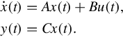
We know there exists a minimal realization for G(s),

$\begin{array}{l} \begin{matrix} \dot{x} (t) = A x (t) + B u (t), \\ y (t) = C x (t) . \end{matrix} \end{array}$ $\begin{array}{l} \begin{matrix} \dot{x} (t) = A x (t) + B u (t), \\ y (t) = C x (t) . \end{matrix} \end{array}$

si128_e (4.43)

In exploring the connection between a transfer function and its minimal realizations, an additional bit of terminology is convenient.

Definition 4.5.1

Suppose N(s)D⁻¹(s) is a coprime right polynomial fraction description for the p × m, strictly proper, rational transfer function G(s). Then the degree of this polynomial fraction description is called the McMillan degree of G(s).

The first objective is to show that the McMillan degree of G(s) is precisely the dimension of minimal realizations of G(s). Our roundabout strategy is to prove that minimal realizations cannot have dimension less than the McMillan degree, and then compute a realization of dimension equal to the McMillan degree. This forces the conclusion that the computed realization is a minimal realization.

Lemma 4.5.1

The dimension of any realization of a strictly proper rational transfer function G(s) is at least the McMillan degree of G(s).

Proof

Suppose that the linear state equation (4.43) is a dimension-n minimal realization for the p × m transfer function G(s). Then Eq. (4.43) is both controllable and observable, and

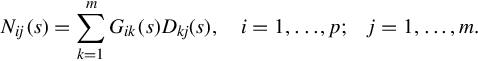
$\begin{array}{l} G (s) = C {(s I - A)}^{- 1} B . \end{array}$ $\begin{array}{l} G (s) = C {(s I - A)}^{- 1} B . \end{array}$

Define a n × m strictly proper transfer function H(s) by the left polynomial fraction description

$\begin{array}{l} H (s) = D_{L}^{- 1} (s) N_{L} (s) = {(s I - A)}^{- 1} B . \end{array}$ $\begin{array}{l} H (s) = D_{L}^{- 1} (s) N_{L} (s) = {(s I - A)}^{- 1} B . \end{array}$

(4.44)

Clearly this left polynomial fraction description has degree n. Since the state equation (4.43) is controllable, then

$\begin{array}{l} \begin{matrix} rank [D_{L} (s_{0})] N_{L} (s_{0})] & = rank [(s_{0} I - A) B] \\ = n \end{matrix} \end{array}$ $\begin{array}{l} \begin{matrix} rank [D_{L} (s_{0})] N_{L} (s_{0})] & = rank [(s_{0} I - A) B] \\ = n \end{matrix} \end{array}$

(4.45)

for every complex s₀. Thus by Theorem 4.3.3 the left polynomial fraction description (4.44) is coprime. Now suppose $N_{a} (s) D_{a}^{- 1} (s)$ $N_{a} (s) D_{a}^{- 1} (s)$ is a coprime right polynomial fraction description for H(s). Then this right polynomial fraction description also has degree n, and

$\begin{array}{l} G (s) = [C N_{a} (s)] D_{a}^{- 1} (s) \end{array}$ $\begin{array}{l} G (s) = [C N_{a} (s)] D_{a}^{- 1} (s) \end{array}$

(4.46)

is a degree-n right polynomial fraction description for G(s), though not necessarily coprime. Therefore the McMillan degree of G(s) is no greater than n, the dimension of a minimal realization of G(s).

For notational assistance in the construction of a minimal realization, recall the integrator coefficient matrices corresponding to a set of k positive integers, α₁, …, α_k, with α₁ + ⋯ + α_k = n. These matrices are

$\begin{array}{l} A_{0} = b l o c k d i a g o n a l \{\begin{array}{l} {[\begin{array}{l} 0 & 1 & \dots & 0 \\ 0 & 0 & \dots & 0 \\ ⋮ & ⋮ & ⋮ & ⋮ \\ 0 & 0 & \dots & 1 \\ 0 & 0 & \dots & 0 \end{array}]}_{(α_{i} \times α_{i})} & , & i = 1, \dots, k \end{array}\}, \end{array}$ $\begin{array}{l} A_{0} = b l o c k d i a g o n a l \{\begin{array}{l} {[\begin{array}{l} 0 & 1 & \dots & 0 \\ 0 & 0 & \dots & 0 \\ ⋮ & ⋮ & ⋮ & ⋮ \\ 0 & 0 & \dots & 1 \\ 0 & 0 & \dots & 0 \end{array}]}_{(α_{i} \times α_{i})} & , & i = 1, \dots, k \end{array}\}, \end{array}$

si134_e (4.47)

$\begin{array}{l} B_{0} = b l o c k d i a g o n a l \{\begin{array}{l} {[\begin{array}{l} 0 \\ ⋮ \\ 0 \\ 1 \end{array}]}_{(α_{i} \times 1)} & , & i = 1, \dots, k \end{array}\} . \end{array}$ $\begin{array}{l} B_{0} = b l o c k d i a g o n a l \{\begin{array}{l} {[\begin{array}{l} 0 \\ ⋮ \\ 0 \\ 1 \end{array}]}_{(α_{i} \times 1)} & , & i = 1, \dots, k \end{array}\} . \end{array}$

si135_e (4.48)

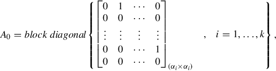
Define the corresponding integrator polynomial matrices by

$\begin{array}{l} ψ (s) = b l o c k d i a g o n a l \{\begin{array}{l} [\begin{array}{l} 1 \\ s \\ ⋮ \\ s^{α_{i} - 1} \end{array}] & , & i = 1, \dots, k \end{array}\}, \end{array}$ $\begin{array}{l} ψ (s) = b l o c k d i a g o n a l \{\begin{array}{l} [\begin{array}{l} 1 \\ s \\ ⋮ \\ s^{α_{i} - 1} \end{array}] & , & i = 1, \dots, k \end{array}\}, \end{array}$

si136_e (4.49)

$\begin{array}{l} Δ (s) = d i a g o n a l {s^{α_{1}}, \dots, s^{α_{k}}} . \end{array}$ $\begin{array}{l} Δ (s) = d i a g o n a l {s^{α_{1}}, \dots, s^{α_{k}}} . \end{array}$

(4.50)

The terminology couldn’t be more appropriate, as we now demonstrate.

Lemma 4.5.2

The integrator polynomial matrices provide a right polynomial fraction description for the corresponding integrator state equation. That is,

$\begin{array}{l} {(s I - A_{0})}^{- 1} B_{0} = ψ (s) Δ^{- 1} (s) . \end{array}$ $\begin{array}{l} {(s I - A_{0})}^{- 1} B_{0} = ψ (s) Δ^{- 1} (s) . \end{array}$

(4.51)

Proof

To verify Eq. (4.51), first multiply on the left by (sI − A₀) and on the right by Δ(s) to obtain

$\begin{array}{l} B_{0} Δ (s) = s ψ (s) - A_{0} ψ (s) . \end{array}$ $\begin{array}{l} B_{0} Δ (s) = s ψ (s) - A_{0} ψ (s) . \end{array}$

(4.52)

This expression is easy to check in a column-by-column fashion using the structure of the various matrices. For example the first column of Eq. (4.52) is the obvious

$\begin{array}{l} [\begin{array}{l} 0 \\ ⋮ \\ 0 \\ s^{α_{1}} \\ 0 \\ ⋮ \\ 0 \end{array}] = [\begin{array}{l} s \\ ⋮ \\ s^{α_{1} - 1} \\ s^{α_{1}} \\ 0 \\ ⋮ \\ 0 \end{array}] - [\begin{array}{l} s \\ ⋮ \\ s^{α_{1} - 1} \\ 0 \\ 0 \\ ⋮ \\ 0 \end{array}] . \end{array}$ $\begin{array}{l} [\begin{array}{l} 0 \\ ⋮ \\ 0 \\ s^{α_{1}} \\ 0 \\ ⋮ \\ 0 \end{array}] = [\begin{array}{l} s \\ ⋮ \\ s^{α_{1} - 1} \\ s^{α_{1}} \\ 0 \\ ⋮ \\ 0 \end{array}] - [\begin{array}{l} s \\ ⋮ \\ s^{α_{1} - 1} \\ 0 \\ 0 \\ ⋮ \\ 0 \end{array}] . \end{array}$

si140_e (4.53)

Proceeding similarly through the remaining columns in Eq. (4.52) yields the proof.

Completing our minimal realization strategy now reduces to comparing a special representation for the polynomial fraction description and a special structure for a dimension-n state equation.

Theorem 4.5.1

Suppose that a strictly proper rational transfer function is described by a coprime right polynomial fraction description (4.42), where D(s) is column reduced with column degrees c₁[D], …, c_m[D] ≥ 1. Then the McMillan degree of G(s) is given by n = c₁[D] + ⋯ + c_m[D], and minimal realizations of G(s) have dimension n. Furthermore, writing

$\begin{array}{l} \begin{matrix} N (s) = N_{l} ψ (s) \\ D (s) = D_{h c} Δ (s) + D_{l} ψ (s), \end{matrix} \end{array}$ $\begin{array}{l} \begin{matrix} N (s) = N_{l} ψ (s) \\ D (s) = D_{h c} Δ (s) + D_{l} ψ (s), \end{matrix} \end{array}$

si141_e (4.54)

where ψ(s) and Δ(s) are the integrator polynomial matrices corresponding to c₁[D], …, c_m[D], a minimal realization for G(s) is

$\begin{array}{l} \begin{matrix} \dot{x} (t) = (A_{0} - B_{0} D_{h c}^{- 1} D_{l}) x (t) + B_{0} D_{h c}^{- 1} u (t) \\ y (t) = N_{l} x (t), \end{matrix} \end{array}$ $\begin{array}{l} \begin{matrix} \dot{x} (t) = (A_{0} - B_{0} D_{h c}^{- 1} D_{l}) x (t) + B_{0} D_{h c}^{- 1} u (t) \\ y (t) = N_{l} x (t), \end{matrix} \end{array}$

si142_e (4.55)

where A₀ and B₀ are the integrator coefficient matrices corresponding to c₁[D], …, c_m[D].

Proof

First we verify that Eq. (4.55) is a realization for G(s). It is straightforward to write down the representation in Eq. (4.54), where N_l and D_l are constant matrices that select for appropriate polynomial entries of N(s), and D_l(s). Then solving for Δ(s) in Eq. (4.54) and substituting into Eq. (4.52) gives

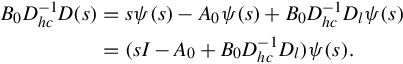
$\begin{array}{l} \begin{matrix} B_{0} D_{h c}^{- 1} D (s) & = s ψ (s) - A_{0} ψ (s) + B_{0} D_{h c}^{- 1} D_{l} ψ (s) \\ = (s I - A_{0} + B_{0} D_{h c}^{- 1} D_{l}) ψ (s) . \end{matrix} \end{array}$ $\begin{array}{l} \begin{matrix} B_{0} D_{h c}^{- 1} D (s) & = s ψ (s) - A_{0} ψ (s) + B_{0} D_{h c}^{- 1} D_{l} ψ (s) \\ = (s I - A_{0} + B_{0} D_{h c}^{- 1} D_{l}) ψ (s) . \end{matrix} \end{array}$

si143_e (4.56)

This implies

$\begin{array}{l} {(s I - A_{0} + B_{0} D_{h c}^{- 1} D_{l})}^{- 1} B_{0} D_{h c}^{- 1} = ψ (s) D^{- 1} (s) \end{array}$ $\begin{array}{l} {(s I - A_{0} + B_{0} D_{h c}^{- 1} D_{l})}^{- 1} B_{0} D_{h c}^{- 1} = ψ (s) D^{- 1} (s) \end{array}$

(4.57)

from which the transfer function for Eq. (4.55) is

$\begin{array}{l} N_{l} {(s I - A_{0} + B_{0} D_{h c}^{- 1} D_{l})}^{- 1} B_{0} D_{h c}^{- 1} = N (s) D^{- 1} (s) . \end{array}$ $\begin{array}{l} N_{l} {(s I - A_{0} + B_{0} D_{h c}^{- 1} D_{l})}^{- 1} B_{0} D_{h c}^{- 1} = N (s) D^{- 1} (s) . \end{array}$

(4.58)

Thus Eq. (4.55) is a realization of G(s) with dimension c₁[D] + ⋯ + c_m[D], which is the McMillan degree of G(s). Then by invoking Lemma 4.5.1 we conclude that the McMillan degree of G(s) is the dimension of minimal realizations of G(s).

In the minimal realization (4.55), note that if D_hc is upper triangular with unity diagonal entries, then the realization is in the controller form. (Upper triangular structure for D_hc can be obtained by elementary column operations on the original polynomial fraction description.) If Eq. (4.55) is in controller form, then the controllability indices are precisely ρ₁ = c₁[D], …, ρ_m = c_m[D]. We see that all minimal realizations of N(s)D⁻¹(s) have the same controllability indices up to reordering. All minimal realizations of a strictly proper rational transfer function G(s) have the same controllability indices up to reordering.

Calculations similar to those in the proof of Theorem 4.5.1 can be used to display a right polynomial fraction description for a given linear state equation.

Theorem 4.5.2

Suppose the linear state equation (4.43) is controllable with controllability indices ρ₁, …, ρ_m ≥ 1. Then the transfer function for Eq. (4.43) is given by the right polynomial fraction description

$\begin{array}{l} C {(s I - A)}^{- 1} B = N (s) D^{- 1} (s), \end{array}$ $\begin{array}{l} C {(s I - A)}^{- 1} B = N (s) D^{- 1} (s), \end{array}$

(4.59)

where

$\begin{array}{l} \begin{matrix} N (s) = C P^{- 1} ψ (s) \\ D (s) = R^{- 1} Δ (s) - R^{- 1} U P^{- 1} ψ (s) \end{matrix} \end{array}$ $\begin{array}{l} \begin{matrix} N (s) = C P^{- 1} ψ (s) \\ D (s) = R^{- 1} Δ (s) - R^{- 1} U P^{- 1} ψ (s) \end{matrix} \end{array}$

si147_e (4.60)

and D(s) is column reduced. Here ψ(s) and Δ(s) are the integrator polynomial matrices corresponding to ρ₁, …, ρ_m, P is the controller-form variable change, and U and R are the coefficient matrices. If the state equation (4.43) also is observable, then N(s)D⁻¹(s) is coprime with degree n.

Proof

We can write

$\begin{array}{l} P A P^{- 1} = A_{0} + B_{0} U P^{- 1}, P B = B_{0} R, \end{array}$ $\begin{array}{l} P A P^{- 1} = A_{0} + B_{0} U P^{- 1}, P B = B_{0} R, \end{array}$

(4.61)

where A₀ and B₀ are the integrator coefficient matrices corresponding to ρ₁, …, ρ_m. Let Δ(s) and ψ(s) be the corresponding integrator polynomial matrices. Using Eq. (4.60) to substitute for Δ(s) in Eq. (4.52) gives

$\begin{array}{l} B_{0} R D (s) + B_{0} U P^{- 1} ψ (s) = s ψ (s) - A_{0} ψ (s) . \end{array}$ $\begin{array}{l} B_{0} R D (s) + B_{0} U P^{- 1} ψ (s) = s ψ (s) - A_{0} ψ (s) . \end{array}$

(4.62)

Rearranging this expression yields

$\begin{array}{l} ψ (s) D^{- 1} (s) = {(s I - A_{0} - B_{0} U P^{- 1})}^{- 1} B_{0} R \end{array}$ $\begin{array}{l} ψ (s) D^{- 1} (s) = {(s I - A_{0} - B_{0} U P^{- 1})}^{- 1} B_{0} R \end{array}$

(4.63)

and therefore

$\begin{array}{l} \begin{matrix} N (s) D^{- 1} (s) & = C P^{- 1} {(s I - A_{0} - B_{0} U P^{- 1})}^{- 1} B_{0} R \\ = C P^{- 1} {(s I - P A P^{- 1})}^{- 1} P B \\ = C {(s I - A)}^{- 1} B . \end{matrix} \end{array}$ $\begin{array}{l} \begin{matrix} N (s) D^{- 1} (s) & = C P^{- 1} {(s I - A_{0} - B_{0} U P^{- 1})}^{- 1} B_{0} R \\ = C P^{- 1} {(s I - P A P^{- 1})}^{- 1} P B \\ = C {(s I - A)}^{- 1} B . \end{matrix} \end{array}$

si151_e (4.64)

This calculation verifies that the polynomial fraction description defined by Eq. (4.60) represents the transfer function of the linear state equation (4.43). Also, D(s) in Eq. (4.60) is column reduced because D_hc = R⁻¹. Since the degree of the polynomial fraction description is n, if the state equation also is observable, hence a minimal realization of its transfer function, then n is the McMillan degree of the polynomial fraction description (4.60).

For left polynomial fraction descriptions, the strategy for right fraction descriptions applies since the McMillan degree of G(s) also is the degree of any coprime left polynomial fraction description for G(s). The only details that remain in proving a left-handed version of Theorem 4.5.1 involve construction of a minimal realization. But this construction is not difficult to deduce from a summary statement.

Theorem 4.5.3

Suppose that a strictly proper rational transfer function is described by a coprime left polynomial fraction description D⁻¹(s)N(s), where D(s) is row reduced with row degrees r₁[D], …, r_p[D] ≥ 1. Then the McMillan degree of G(s) is given by n = r₁[D] + ⋯ + r_p[D], and minimal realizations of G(s) have dimension n. Furthermore, writing

$\begin{array}{l} \begin{matrix} N (s) = ψ^{T} (s) N_{l} \\ D (s) = Δ (s) D_{h r} + ψ^{T} (s) D_{l}, \end{matrix} \end{array}$ $\begin{array}{l} \begin{matrix} N (s) = ψ^{T} (s) N_{l} \\ D (s) = Δ (s) D_{h r} + ψ^{T} (s) D_{l}, \end{matrix} \end{array}$

si152_e (4.65)

where ψ(s) and Δ(s) are the integrator polynomial matrices corresponding to r₁[D], …, r_p[D], a minimal realization for G(s) is

$\begin{array}{l} \begin{matrix} \dot{x} (t) = (A_{0}^{T} - D_{l} D_{h r}^{- 1} B_{0}^{T}) x (t) + N_{l} u (t) \\ y (t) = D_{h r}^{- 1} B_{0}^{T} x (t), \end{matrix} \end{array}$ $\begin{array}{l} \begin{matrix} \dot{x} (t) = (A_{0}^{T} - D_{l} D_{h r}^{- 1} B_{0}^{T}) x (t) + N_{l} u (t) \\ y (t) = D_{h r}^{- 1} B_{0}^{T} x (t), \end{matrix} \end{array}$

si153_e (4.66)

where A₀ and B₀ are the integrator coefficient matrices corresponding to r₁[D], …, r_p[D].

Analogous to the discussion following Theorem 4.5.3, in the setting of Theorem 4.5.3 the observability indices of minimal realizations of D⁻¹(s)N(s) are the same, up to reordering, as the row degrees of D(s).

Theorem 4.5.4

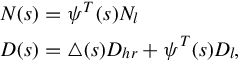
Suppose the linear state equation (4.43) is observable with observability indices η₁, …, η_p ≥ 1. Then the transfer function for Eq. (4.43) is given by the left polynomial fraction description

$\begin{array}{l} C {(s I - A)}^{- 1} B = D^{- 1} (s) N (s), \end{array}$ $\begin{array}{l} C {(s I - A)}^{- 1} B = D^{- 1} (s) N (s), \end{array}$

where

$\begin{array}{l} N (s) = ψ^{T} (s) Q^{- 1} B, \\ D (s) = Δ (s) S^{- 1} - ψ^{T} (s) Q^{- 1} V S^{- 1} \end{array}$ $\begin{array}{l} N (s) = ψ^{T} (s) Q^{- 1} B, \\ D (s) = Δ (s) S^{- 1} - ψ^{T} (s) Q^{- 1} V S^{- 1} \end{array}$

si155_e (4.67)

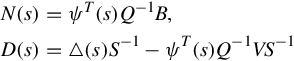
and D(s) is row reduced. Here ψ(s) and Δ(s) are the integrator polynomial matrices corresponding to η₁, …, η_p, Q is the observer-form variable change, and V and S are the coefficient matrices. If the state equation (4.43) also is controllable, then D⁻¹(s)N(s) is coprime with degree n.

..................Content has been hidden....................

You can't read the all page of ebook, please click here login for view all page.

Table of Contents for 4: Polynomial fraction description

Create new playlist

Sign In

Sign Up

4.1 Introduction

4.2 Right polynomial fractions

4.3 Left polynomial fraction

4.4 Column and row degrees

4.5 Minimal realization

Table of Contents for
4: Polynomial fraction description