
Mathematical preliminaries
Keywords
Vector algebra; Matrix algebra; Linear differential equation; Matrix differential equation; Laplace transform; Solution to linear equations; Solution to matrix ordinary differential equations; Stability
In this chapter, we briefly discuss some basic topics in linear algebra that may be needed in the sequel. This chapter can be skimmed very quickly and used mainly as a quick reference. There has been a huge number of reference resources for matrix and linear algebra, to mention a few [43–50].
2.1 Vector algebra
If one measures a physical quantity, one will obtain a number or a sequence of numbers in a particular order. This is the so-called scalar, which is a single number quantity, and one can use it to gauge the magnitude or the value of the measurement. Scalars can be compared only if they have the same units. For example, we can compare a speed in km/h with another speed in km/h but we cannot compare a speed with a density because they are in different units.
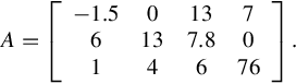
An array is defined as a sequence of scalar numbers in a certain order. A rectangular table, which consists of an array of arrays, that are arranged in terms of a certain rule, is called a matrix. A matrix consists of m rows and n columns. For instance, the following is a 3 × 4 real matrix:
A special case of a matrix where it has only one row or one column is called a vector. Before we present the definition of a vector, let us take a look from how we distinct an array and a vector from computational point of view. A vector is usually used as a quantity that requires both magnitude and direction in space. Examples of vector can be displacement, velocity, acceleration, force, momentum, electric field, the traffic load in links of Internet, and so on. Vectors can be compared if they have the same physical units and geometrical dimensions. For instance, you can compare two-dimensional force with another two-dimensional force but you cannot compare two-dimensional force with three-dimensional force. Similarly, you cannot compare force with velocity because they have different physical units. You cannot compare the routing matrix with a traffic matrix in Internet because they are of different philosophy.
The total number of elements in a vector is called the dimension or the size of the vector. Since a vector can have a number of elements, we say that the space where the vector lies is a multidimensional space with the specific dimensions.
The magnitude of a vector is sometimes called the length of a vector, or norm of a vector. The direction of a vector in space is measured from another vector (i.e., standard basis vector), represented by the cosine angle between the two vectors.
Unlike ordinary arrays, vectors are special and can be viewed from both an algebraic and a geometric point of view. Algebraically, a vector is just an array of scalar elements. From a computational point of view, a vector is represented as a two-dimensional array while an ordinary array is represented as a one-dimensional array.
There are rich implications for vectors in geometry. A vector can also be represented as a point in space. When a vector is represented as a point in space, we can also view that vector as an arrow starting at the origin of a coordinate system pointing toward the destination point. Because the coordinate system does not change, we only need to draw the points without the arrows. In a geometrical diagram, a vector is usually plotted as an arrow in space, which can be translated along the line containing it. Subsequently, the vector can also be applied to any point in space if the magnitude and direction of both do not change.
2.2 Matrix algebra
2.2.1 Matrix properties
Determinant: Each n × n square matrix A has an associated scalar number, which is termed as the determinant of that matrix and is noted either by ![]() or by |A|. This value determines whether the matrix has an inverse or not.
or by |A|. This value determines whether the matrix has an inverse or not.
When the matrix order is 1, That is, A1×1 = [a] then we calculate its determinant as |A| = a.
When the matrix order is 2, that is

then we have

When the matrix order is 3,
then we compute the determinant by the following formula:

In general, when we have the following general order of matrix An×n = [aij], then we define the following components:
• The minor of [aij] is the determinant of an (n − 1) × (n − 1) submatrix denoted by Mij. The submatrix Mij is then obtained from the matrix An×n by deleting the row and column containing the element aij.
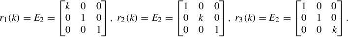
• The signed minor is called cofactor of aij denoted by Aij. The cofactor is a scalar sign being determined by ![]() This sign follows the following order:
This sign follows the following order:

• The determinant of matrix An×n = [aij] is the summed product of the first column entries with its cofactor. That is,
Matrix trace: Trace of a square matrix is the summation of matrix diagonal entries ![]() . Trace of a matrix is also called spur of a square matrix. For square matrices A and B, it is true that
. Trace of a matrix is also called spur of a square matrix. For square matrices A and B, it is true that

where AT denotes the transpose. The trace is also invariant under a similarity transformation, i.e., if
we have
The trace of a product of two square matrices is independent of the order of the multiplication. That is, we have
Therefore, the trace of the commutator of A and B is given by
The trace of a product of three or more square matrices, on the other hand, is invariant only under cyclic permutations of the order of multiplication of the matrices, by a similar argument. The product of a symmetric and an antisymmetric matrix has zero trace, i.e.,
Matrix rank: The dimension of row space of a matrix is equal to the dimension of the column space of that matrix. The common dimension of the row space and column space of matrix A is defined as the rank of matrix A, denoted by rank(A) = R(A). It is seen that the rank of a matrix is the number of linearly independent vectors and equal to the dimension of space spanned by those vectors. To put it in another way, the rank of A is the number of basis vectors we can form from matrix A, because performing an elementary row operation does not change the row space. To compute the rank of a matrix, we usually perform manipulations on the matrix to bring it into the so-called reduced row echelon form (RREF, also called row canonical form) and subsequently the nonzero rows of the RREF matrix will form the basis for the row space.
A matrix is in RREF if it satisfies the following conditions:
• It is in row echelon form (REF).
• Every leading coefficient is 1 and is the only nonzero entry in its column.
The RREF of a matrix may be computed by Gauss-Jordan elimination. Unlike the REF, the RREF of a matrix is unique and does not depend on the algorithm used to compute it.
The following matrix is an example of one in RREF:

Note that this does not always mean that the left of the matrix will be an identity matrix, as this example shows.
For matrices with integer coefficients, the Hermite normal form is an REF that may be calculated using Euclidean division and without introducing any rational number or denominator. On the other hand, the reduced echelon form of a matrix with integer coefficients generally contains noninteger entries.
We assume that A is an m × n matrix, and we define the linear map f by f(x) = Ax. The rank of an m × n matrix is a nonnegative integer and cannot be greater than either m or n, that is,
A matrix that has rank ![]() is said to have full rank; otherwise, the matrix is rank deficient. Note that only a zero matrix has rank zero. f is injective (or “one-to-one”) if and only if A has rank n (in this case, we say that A has full column rank), while f is surjective (or “onto”) if and only if A has rank m (in this case, we say that A has full row rank). If A is a square matrix (i.e., m = n), then A is invertible if and only if A has rank n (i.e., A has full rank). If B is any n × k matrix, then
is said to have full rank; otherwise, the matrix is rank deficient. Note that only a zero matrix has rank zero. f is injective (or “one-to-one”) if and only if A has rank n (in this case, we say that A has full column rank), while f is surjective (or “onto”) if and only if A has rank m (in this case, we say that A has full row rank). If A is a square matrix (i.e., m = n), then A is invertible if and only if A has rank n (i.e., A has full rank). If B is any n × k matrix, then
If B is an n × k matrix of rank n, then
If C is an l × m matrix of rank m, then
The rank of A is equal to r if and only if there exists an invertible m × m matrix X and an invertible n × n matrix Y such that

where Ir denotes the r × r identity matrix.
Sylvesters rank inequality: if A is an m × n matrix and B is n × k, then
This is a special case of the next inequality. The inequality due to Frobenius: if AB, ABC, and BC are defined, then
Subadditivity:
when A and B are of the same dimension. As a consequence, a rank-k matrix can be written as the sum of k rank-1 matrices, but not fewer. The rank of a matrix plus the nullity of the matrix equals to the number of columns of the matrix. (This is the well-known rank-nullity theorem.) If A is a matrix over the real numbers then the rank of A and the rank of its corresponding Gram matrix are equal. Thus, for real matrices
This can be shown by proving equality of their null spaces. The null space of the Gram matrix is given by vectors x for which ATAx = 0. If this condition is fulfilled, we also have ![]() If A is a matrix over the complex numbers and A* denotes the conjugate transpose of A, then one has
If A is a matrix over the complex numbers and A* denotes the conjugate transpose of A, then one has
2.2.2 Basic matrix operations
Matrix transpose: Transpose of a matrix is obtained by interchanging all rows with all columns of the matrix. If the matrix size is m × n, the transpose matrix size is n × m.
Matrix addition: If two matrices are of the same order, we then take the summation of any pair of elements, which are at the same position in a peer-to-peer manner in these two matrices to yield the summation. Namely, for two matrices A and B, then the sum of the two matrices C = A + B is a matrix whose entry is equal to the sum of the corresponding entries cij = aij + bij.
Matrix subtraction: When we have two matrices, A and B then the matrix subtraction or matrix difference C = A − B is a matrix whose entry is formed by subtracting the corresponding entry of B from each entry of A, that is cij = aij − bij. Matrix subtraction works only when the two matrices have the same size and the result is also the same size as the original matrices.
Matrix multiplication: One of the most important matrix operations is matrix multiplication or matrix product. The multiplication of two matrices A and B is a matrix C = A × B whose element cij consists of the vector inner product of the ith row of matrix A and the jth column of matrix B, that is ![]() . Matrix multiplication can be done only when the number of column of A is equal to the number of rows of B. If the size of matrix A is m × n and the size of matrix B is n × p, then the result of matrix multiplication is a matrix size m by p, or in short Am×nBn×p = Cm×p.
. Matrix multiplication can be done only when the number of column of A is equal to the number of rows of B. If the size of matrix A is m × n and the size of matrix B is n × p, then the result of matrix multiplication is a matrix size m by p, or in short Am×nBn×p = Cm×p.
Matrix scalar multiple: When we multiply a real number k with a matrix A, we have the scalar multiple of A. The scalar multiple matrix B = kA has the same size of the matrix A and it is obtained by multiplying each element of A by k. That is bij = kaij.
Hadamard product: Matrix element-wise product is also called Hadamard product or direct product. It is a direct element by element multiplication. If matrix C = AB is the direct product two matrices A and B, then the element of Hadamard product is simply cij = aij × bij. The direct product has the same size as the original matrices.
Horizontal concatenation: It is often useful to think of a matrix composed of two or more submatrices or a block of matrices. A matrix can be partitioned into smaller matrices by setting a horizontal line or a vertical line. For example

Matrix horizontal concatenation is an operation to join two sub matrices horizontally into one matrix. This is the reverse operation of partitioning.
Vertical concatenation: Matrix vertical concatenation is an operation to join two sub matrices vertically into one matrix.
Elementary row operation: In linear algebra, there are three elementary row operations. The same operations can also be used for column (simply by changing the word row into column). The elementary row operations can be applied to a rectangular matrix size m × n:
1. interchanging two rows of the matrix;
2. multiplying a row of the matrix by a scalar;
3. add a scalar multiple of a row to another row.
Applying the above three elementary row operations to a matrix will produce a row equivalent matrix. When we view a matrix as the augmented matrix of a linear system, the three elementary row operations are equivalent to interchanging two equations, multiplying an equation by a nonzero constant and adding a scalar multiple of one equation to another equation. Two linear systems are equivalent if they produce the same set of solutions. Since a matrix can be seen as a linear system, applying the above three elementary row operations does not change the solutions of that matrix. The three elementary row operations can be put into three elementary matrices. Elementary matrix is a matrix formed by performing a single elementary row operation on an identity matrix. Multiplying the elementary matrix to a matrix will produce the row equivalent matrix based on the corresponding elementary row operation.
Elementary Matrix Type 1: Interchanging two rows of the matrix

Elementary Matrix Type 2: Multiplying a row of the matrix by a scalar
Elementary Matrix Type 3: Add a scalar multiple of a row to another row

Reduced row echelon form: There is a standard form of a row equivalent matrix and if we do a sequence of row elementary operations to reach this standard form we may gain the solution of the linear system. The standard form is called RREF of a matrix, or matrix RREF in short. An m × n matrix is called to be in an RREF when it satisfies the following conditions:
1. All zero rows, if any, are at the bottom of the matrix.
2. Reading from left to right, the first non zero entry in each row that does not consist entirely of zeros is a 1, called the leading entry of its row.
3. If two successive rows do not consist entirely of zeros, the second row starts with more zeros than the first (the leading entry of second row is to the right of the leading entry of first row).
4. All other elements of the column in which the leading entry 1 occurs are zeros.
When only the first three conditions are satisfied, the matrix is called in Row Echelon Form (REF). Using Reduced Row Echelon Form of a matrix we can calculate matrix inverse, rank of matrix, and solve simultaneous linear equations.
Finding inverse using RREF (Gauss-Jordan): We can use the three elementary row operations to find the row equivalent of RREF of a matrix. Using the Gauss-Jordan method, you can obtain matrix inverse. Gauss-Jordan method is based on the following theorem: A square matrix is invertible if and only if it is row equivalent to the identity matrix. The method to find inverse using the Gauss-Jordan method is as follows:
• we concatenate the original matrix with the identity matrix;
• perform the row elementary operations to reach RREF;
• if the left part of the matrix RREF is equal to an identity matrix, then the left part is the inverse matrix;
• if the left part of the matrix RREF is not equal to an identity matrix, then we conclude the original matrix is singular. It has no inverse.
Finding a matrix’s rank using RREF: Another application of elementary row operations to find the row equivalent of RREF of the matrix is to find matrix rank. Similar to trace and determinant, the rank of a matrix is a scalar number showing the number of linearly independent vectors in a matrix, or the order of the largest square submatrix of the original matrix whose determinant is nonzero. To compute the rank of a matrix through elementary row operations, simply perform the elementary row operations until the matrix reach the RREF. Then the number of nonzero rows indicates the rank of the matrix.
Singular matrix: A square matrix is singular if the matrix has no inverse. To determine whether a matrix is singular or not, we simply compute the determinant of the matrix. If the determinant is zero, then the matrix is singular.
2.3 Matrix inverse
When we are dealing with ordinary number, when we say ab = 1 then we can obtain b = 1/a as long as b≠0. We write it as b = a−1 or aa−1 = a−1a = 1. Matrix inverse is similar to division operation in ordinary numbers. Suppose we have matrix multiplication such that the result of matrix product is an identity matrix AB = I. If such matrix B exists, then that matrix is unique and we can write B = A−1 or we can also write AA−1 = I = A−1A.
Matrix inverse exists only for a square matrix (that is a matrix having the same number of rows and columns). Unfortunately, matrix inverse does not always exist. Thus, we term that a square matrix is singular if that matrix does not have an inverse, it is called nonregular matrix as well. Because matrix inverse is a very important operation, in linear algebra, there are many ways to compute matrix inverse:
1. The simplest way to find matrix inverse for a small matrix (order 2 or 3) is to use Cramers rule that employs the determinant of the original matrix. Recall that a square matrix is singular (i.e., no inverse) if and only if the determinant is zero. The matrix inverse can be computed by scaling the adjoint of the original matrix with the determinant. That is,
The adjoint of a matrix is the one whose element is the cofactor of the original matrix. For a 2 by 2 matrix
we have

The determinant is set by multiplying the diagonal elements minus the product of the off-diagonal elements and the adjoint is set by reversing the diagonal elements and taking the minus sign of the off diagonal elements.
2. For a matrix of medium size (order 4–10), the usage of elementary row operations to produce RREF matrix using Gaussian Elimination or Gauss-Jordan is useful.
3. Other techniques to compute matrix inverse of medium to large size are to use numerical methods such as LU decomposition, singular value decomposition (SVD), or the Monte Carlo method.
4. For a large square matrix (order more than 100), numerical techniques such as the Gauss-Siedel, Jacobi method, Newton’s method, the Cayley-Hamilton method, eigenvalue decomposition and Cholesky decomposition are used to calculate the matrix inverse accurately or approximately.
5. For a partitioned block matrix with 2 × 2 blocks, we have some specific method to compute its inverse, as outlined in the sequel.
We briefly introduce the following specific methods for computing the inverse of a matrix:
Gaussian elimination: Gauss-Jordan elimination is an algorithm that can be used to determine whether a given matrix is invertible and to find the inverse. An alternative is the LU decomposition, which generates upper and lower triangular matrices that are easier to invert.
Newton’s method: Newton’s method as used for a multiplicative inverse algorithm may be convenient, if it is possible to find a suitable starting seed such that
Newton’s method is particularly useful when dealing with families of related matrices that behave enough like the sequence manufactured for the homotopic above: sometimes a good starting point for refining an approximation for the new inverse can be the already obtained inverse of a previous matrix that nearly matches the current matrix, e.g., the pair of sequences of inverse matrices used in obtaining matrix square roots by Denman-Beavers iteration; this may need more than one pass of the iteration at each new matrix, if they are not close enough together for just one to be enough. Newton’s method is also useful for making up corrections to an Gauss-Jordan algorithm that has been contaminated by small errors due to imperfect computer arithmetic.
Cayley-Hamilton method: The Cayley-Hamilton theorem allows us to represent the inverse of A in terms of ![]() , traces and powers of A. Particularly, for a matrix A, we have its inverse formulated as follows:
, traces and powers of A. Particularly, for a matrix A, we have its inverse formulated as follows:
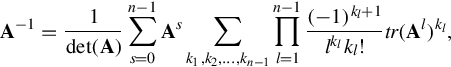
where n is the dimension of A, and tr(A) is the trace of matrix A given by the sum of the main diagonal. The sum is taken over s and the sets of all kl ≥ 0 satisfying the following linear Diophantine equation:
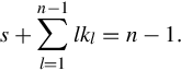
The formula can be rewritten in terms of the complete Bell polynomials of arguments tl = −(l − 1)! tr(Al) as

Eigenvalue decomposition: If matrix A can be eigenvalue decomposed and if none of its eigenvalues are zero, then A is invertible and its inverse is given by
where Q is the square (N × N) matrix whose ith column is the eigenvector qi of A and Λ = [Λii] is the diagonal matrix whose diagonal elements are the corresponding eigenvalues, i.e., Λii = λi. Furthermore, because Λ is a diagonal matrix, its inverse is easy to calculate in the following manner:
Cholesky decomposition: If matrix A is positive definite, then its inverse can be obtained as
where L is the lower triangular Cholesky decomposition of A, and L* denotes the conjugate transpose of L.
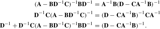
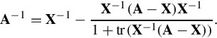
Block-wise inversion: Matrices can also be inverted blockwise by using the following analytic inversion formula:

where A, B, C, and D are block matrices with appropriate sizes. A must be square, so that it can be inverted. Furthermore, A and D − CA−1B must be nonsingular. By this method to compute the block matrix is particularly appealing if A is diagonal and D − CA−1B (the Schur complement of A) is a small matrix, since they are the only matrices requiring inversion.
The nullity theorem says that the nullity of A equals the nullity of the subblock in the lower right of the inverse matrix, whilst the nullity of B equals the nullity of the subblock in the upper right of the inverse matrix.
The inversion procedure leading to Eq. (2.1) is performed in the matrix blocks that is operated on C and D first. Instead, if A and B are operated on first, and provided that D and A − BD−1C are nonsingular, the result is

Equating Eqs. (2.1), (2.2) leads to
which is the Woodbury matrix identity, being equivalent to the binomial inverse theorem, and
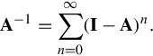
Neumann series: If a matrix A has the property that
then A is nonsingular and its inverse can be expressed by a Neumann series:
Truncating the sum results in an approximate inverse that may be useful as a preconditioner. Note that a truncated series can be accelerated exponentially by noting that the Neumann series is a geometric sum. As such, it satisfies
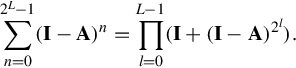
Therefore, only 2L − 2 matrix multiplications are needed to compute 2L terms of the summation. More generally, if A is close to the invertible matrix X in the sense that
then A is nonsingular and its inverse is

If it is also the case that A − X has rank 1 then this is reduced to
Derivative of the matrix inverse: Suppose that the invertible matrix A depends on a parameter t. Then the derivative of the inverse of A with respect to t is given by

Similarly, if ϵ is a small number then
Schur decomposition: The Schur decomposition reads as follows: if A is a n × n square matrix with complex entries, then A can be expressed as
where Q is a unitary matrix (so that its inverse Q−1 is also the conjugate transpose Q * of Q), and U is an upper triangular matrix, which is called a Schur form of A. Since U is similar to A, it has the same multiset of eigenvalues, and since it is triangular, those eigenvalues are the diagonal entries of U.
The Schur decomposition implies that there exists a nested sequence of A-invariant subspaces ![]() and that there exists an ordered orthogonal basis (for the standard Hermitian form of Cn) such that the first i basis vectors span Vi for each i occurring in the nested sequence. In particular, a linear operator J on a complex finite-dimensional vector space stabilizes a complete flag (V1, …, Vn).
and that there exists an ordered orthogonal basis (for the standard Hermitian form of Cn) such that the first i basis vectors span Vi for each i occurring in the nested sequence. In particular, a linear operator J on a complex finite-dimensional vector space stabilizes a complete flag (V1, …, Vn).
Generalized Schur decomposition: Given square matrices A and B, the generalized Schur decomposition factorizes both matrices as A = QSZ* and B = QTZ*, where Q and Z are unitary, and S and T are upper triangular. The generalized Schur decomposition is also sometimes called the QZ decomposition.
The generalized eigenvalues λ that solve the generalized eigenvalue problem Ax = λBx (where x is an unknown nonzero vector) can be calculated as the ratio of the diagonal elements of S to those of T. That is, using subscripts to denote matrix elements, the ith generalized eigenvalue λi satisfies λi = Sii/Tii.
Properties of matrix inverse: Some important properties of matrix inverse are:
• If A and B are square matrices with the order n and their product produces an identity matrix, i.e., A × B = In = B × A, then we have B = A−1.
• If a square matrix A has an inverse (nonsingular), then the inverse matrix is unique.
• A square matrix A has an inverse matrix if and only if the determinant is not zero: |A|≠0. Similarly, the matrix A is singular (has no inverse) if and only if its determinant is zero: |A| = 0.
• A square matrix A with order n has an inverse matrix if and only if the rank of this matrix is full, that is rank(A) = n.
• If a square matrix A has an inverse, the determinant of an inverse matrix is the reciprocal of the matrix determinant. That is ![]()
• If a square matrix A has an inverse, for a scalar k≠0 then the inverse of a scalar multiple is equal to the product of their inverse. That is ![]()
• If a square matrix A has an inverse, the transpose of an inverse matrix is equal to the inverse of the transposed matrix. That is (A−1)T = (AT)−1.
• If A and B are square nonsingular matrices both with the order n then the inverse of their product is equal to the product of their inverse in reverse order. That is (AB)−1 = B−1A−1.
• Let A and B are square matrices with the order n. If A × B = 0 then either A = 0 or B = 0 or both A and B are singular matrices with no inverse.
2.4 Solving system of linear equation
2.4.1 Gauss method
A linear equation in variables x1, x2, …, xn has the form
where the numbers ![]() are the equation’s coefficients and
are the equation’s coefficients and ![]() is a constant. An n-tuple
is a constant. An n-tuple ![]() is a solution of that equation if substituting the numbers s1, s2, …, sn for the variables gives a true statement:
is a solution of that equation if substituting the numbers s1, s2, …, sn for the variables gives a true statement:
A system of linear equations
has the solution (s1, s2, …, sn) if that n-tuple is a solution of all of the equations in the system.
Note that each of the above three operations has a restriction. Multiplying a row by 0 is not allowed because obviously that can change the solution set of the system. Similarly, adding a multiple of a row to itself is not allowed because adding −1 times the row to itself has the effect of multiplying the row by 0. Finally, swap ping a row with itself is disallowed.
2.4.2 A general scheme for solving system of linear equation
Linear equation of system can be written into

The above linear system can be further simplified into a matrix product Ax = b. A solution of linear system is an order collection of n numbers that satisfies the m linear equations, which can be written in short as a vector solution x. A linear system Ax = b is called a nonhomogeneous system when vector b is not a zero vector. A linear system Ax = 0 is called a homogeneous system when the vector b is a zero vector.
Rank of matrix A denoted by R(A) is used to determine whether the linear system is consistent (has a solution), has many solutions or has a unique set of solutions, or inconsistent (has no solution) using matrix inverse. Diagram of Fig. 2.1 shows the solution of the system of linear equations based on rank of the coefficient matrix R(A) in comparison with the matrix size and rank of the augmented matrix coefficients A and the vector constants b: R(A : b).
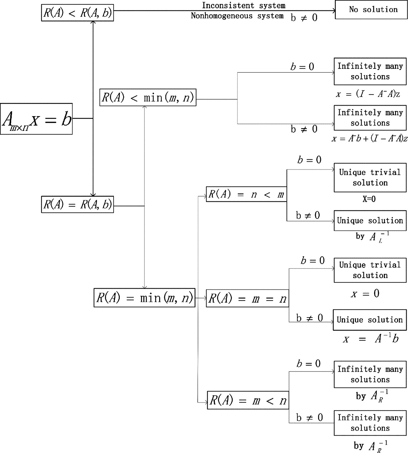
The equation Ax = 0 has infinitely many nontrivia solutions if and only if the matrix coefficient A is singular (i.e., it has no inverse, or ![]() ), which happens when the number of equations is less than the unknowns (m < n). Otherwise, the homogeneous system only has the unique trivial solution of x = 0. General solution for homogeneous system is
), which happens when the number of equations is less than the unknowns (m < n). Otherwise, the homogeneous system only has the unique trivial solution of x = 0. General solution for homogeneous system is
where z is an arbitrary nonzero vector and A− is a generalized inverse ({1}-inverse) matrix of A satisfying AA−A = A.
The linear system Ax = b is called consistent if AA−b = b. A consistent system can be solved using matrix inverse x = A−1b, left inverse ![]() or right inverse
or right inverse ![]() . A full rank nonhomogeneous system (happening when
. A full rank nonhomogeneous system (happening when ![]() ) has three possible options:
) has three possible options:
• When the number of the unknowns in a linear system is the same as the number of equations (m = n), the system is called uniquely determined system. There is only one possible solution to the system computed using matrix inverse x = A−1b.
• When we have more equations than the unknown (m > n), the system is called overdetermined system. The system is usually inconsistent with no possible solution. It is still possible to find unique solution using left inverse ![]() .
.
• When you have more unknowns than the equations (m < n), your system is called an undetermined system. The system usually has many possible solutions. The standard solution can be computed using right inverse ![]() .
.
When a nonhomogeneous system Ax = b is not full rank or when the rank of the matrix coefficients is less than the rank of the augmented coefficients matrix and the vector constants, that is R(A) < R(A : b), then the system is usually inconsistent with no possible solution using matrix inverse. It is still possible to find the approximately least square solution that minimizes the norm of error. That is, using the generalized inverse of the matrix A and by
we obtain
where z is an arbitrary nonzero vector.
2.5 Linear differential equation
2.5.1 Introduction
Linear differential equations are of the form
where the differential operator L is a linear operator, y is the unknown function (such as a function of time y(t)), and the right hand side f is a given function of the same nature as y (called the source term). For a function dependent on time we may write the equation more expressly as
and, even more precisely by bracketing
The linear operator L may be considered to be of the form

The linearity condition on L rules out operations such as taking the square of the derivative of y; but permits, for example, taking the second derivative of y. It is convenient to rewrite this equation in an operator form
where D is the differential operator d/dt (i.e., Dy = y′, D2y = y″, … ), and A1(t), …, An(t) are given functions. Such an equation is said to have order n; the index of the highest derivative of y that is involved.
If y is assumed to be a function of only one variable, one terms it an ordinary differential equation, else the derivatives and their coefficients must be understood as (contracted) vectors, matrices or tensors of higher rank, and we have a (linear) partial differential equation.
The case where f = 0 is called a homogeneous equation and its solutions are called complementary functions. It is particularly important to the solution of the general case, since any complementary function can be added to a solution of the inhomogeneous equation to give another solution (by a method traditionally called particular integral and complementary function). When the components Ai are numbers, the equation is said to have constant coefficients.
2.5.2 Homogeneous equations with constant coefficients
The first method of solving linear homogeneous ordinary differential equations with constant coefficients is due to Euler, who worked out that the solutions have the form ezx, for possibly complex values of z. The exponential function is one of the few functions to keep its shape after differentiation, allowing the sum of its multiple derivatives to cancel out the zeros, as required by the equation. Thus, for constant values A1, …, An, to solve
by setting y = ezx leads to
Division by ezx gives the nth-order polynomial
This algebraic equation F(z) = 0 is the characteristic equation.
Formally, the terms
of the original differential equation are replaced by zk. Solving the polynomial then gives n values of z, z1, …, zn. Substitution of any of those values for z into ezx gives a solution ![]() . Since homogeneous linear differential equations obey the superposition principle, any linear combination of these functions also satisfy the differential equation.
. Since homogeneous linear differential equations obey the superposition principle, any linear combination of these functions also satisfy the differential equation.
When the above roots are all distinct, we have n distinct solutions to the differential equation. It can be shown that these are linearly independent, by applying the Vandermonde determinant, and therefore they form a basis of the space of all solutions of the differential equation.
The procedure gives a solution for the case when all zeros are distinct, that is, each has multiplicity 1. For the general case, if z is a (possibly complex) zero (or root) of F(z) having multiplicity m, then for ![]() , y = xkezx is a solution of the ordinary differential equation. Applying this to all roots gives a collection of n distinct and linearly independent functions, where n is the degree of F(z). As before, these functions make up a basis of the solution space.
, y = xkezx is a solution of the ordinary differential equation. Applying this to all roots gives a collection of n distinct and linearly independent functions, where n is the degree of F(z). As before, these functions make up a basis of the solution space.
If the coefficients Ai of the differential equation are real, then real-valued solutions are generally preferable. Since nonreal roots z then come in conjugate pairs, so do their corresponding basis functions xkezx, and the desired result is obtained by replacing each pair with their real-valued linear combinations Re(y) and Im(y), where y is one of the pair.
A case that involves complex roots can be solved with the aid of Euler’s formula.
Solving of characteristic equation: A characteristic equation also called auxiliary equation of the form
Case 1: Two distinct roots, r1 and r2 .
Case 2: One real repeated root, r.
Case 3: Complex roots, α + βi.
In case 1, the solution is given by
In case 2, the solution is given by
In case 3, using Euler’s equation the solution is given by
2.5.3 Nonhomogeneous equation with constant coefficients
To obtain the solution to the nonhomogeneous equation (sometimes called inhomogeneous equation), find a particular integral yP(x) by either the method of undetermined coefficients or the method of variation of parameters; the general solution to the linear differential equation is the sum of the general solution of the related homogeneous equation and the particular integral. Or, when the initial conditions are set, use Laplace transform to obtain the particular solution directly. Suppose we have

For later convenience, define the characteristic polynomial
We find a solution basis {y1(x), y2(x), …, yn(x)} for the homogeneous (f(x) = 0) case. We now seek a particular integral yp(x) by the variation of parameters method. Let the coefficients of the linear combination be functions of x, for which we formulate
For ease of notation we will drop the dependency on x (i.e., the various (x)). Using the operator notation D = d/dx, the ODE in question is P(D)y = f; so
With the constraints

the parameters commute out,
But P(D)yj = 0, therefore
This, with the constraints, gives a linear system in the uj. Combining the Cramer’s rule with the Wronskian, we have
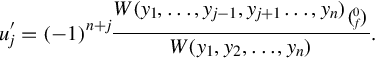
In terms of the nonstandard notation used above, one should take the i, n-minor of W and multiply it by f. That’s why we get a minus-sign. Alternatively, forget about the minus sign and just compute the determinant of the matrix obtained by substituting the jth W column with (0, 0, …, f). The rest is a matter of integrating uj. The particular integral is not unique; yp + c1y1 + ⋯ + cnyn also satisfies the ODE for any set of constants cj.
Example 2.5.1
Suppose we have the following nonhomogeneous deferential equation with constant coefficients
We take the solution basis found above
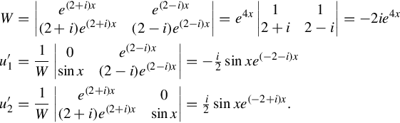
Using the list of integrals of exponential functions
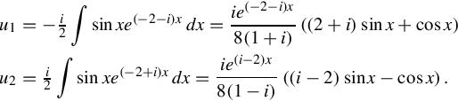
And so

(Notice that u1 and u2 had factors that canceled y1 and y2; that is typical.)
For interest’s sake, this ODE has a physical interpretation as a driven damped harmonic oscillator; yp represents the steady state, and c1y1 + c2y2 is the transient.
2.5.4 Equation with variable coefficients
A linear ODE of order n with variable coefficients has the general form
First-order equation with variable coefficients: A linear ODE of order 1 with variable coefficients has the general form
where D is the differential operator. Equations of this form can be solved by multiplying the integrating factor
throughout to obtain
which simplifies due to the product rule (applied backwards) to
which, on integrating both sides and solving for y(x) gives
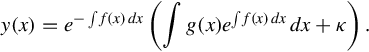
In other words, the solution of a first-order linear ODE
with coefficients, that may or may not vary with x, is

where κ is the constant of integration, and
A compact form of the general solution based on a Green’s function is

where δ(x) is the generalized Dirac delta function.
2.5.5 Systems of linear differential equations
An arbitrary linear ordinary differential equation or even a system of such equations can be converted into a first order system of linear differential equations by adding variables for all but the highest order derivatives. A linear system can be viewed as a single equation with a vector-valued variable. The general treatment is analogous to the treatment above of ordinary first order linear differential equations, but with complications stemming from noncommutativity of matrix multiplication. To solve
where y(x) is a vector or matrix, and A(x) is a matrix, let U(x) be the solution of y′(x) = A(x)y(x) with U(x0) = I (the identity matrix). U is a fundamental matrix for the equation. The columns of U form a complete linearly independent set of solutions for the homogeneous equation. After substituting
the equation
is reduced to
Thus,

If A(x1) commutes with A(x2) for all x1 and x2, then
and thus
However, in the general case there is no closed form solution, and an approximation method such as Magnus expansion may have to be used. Note that the exponentials are matrix exponentials.
2.6 Matrix differential equation
2.6.1 Introduction
A differential equation is a mathematical equation for an unknown function of one or several variables that relates the values of the function itself and of its derivatives of various orders. A matrix differential equation contains more than one function stacked into vector form with a matrix relating the functions to their derivatives. For example, a simple matrix ordinary differential equation is
where x(t) is an n × 1 vector of functions of an underlying variable t, x′(t) is the vector of first derivatives of these functions, and A is a matrix, of which all elements are constants.
In the case where A has n distinct eigenvalues, this differential equation has the following general solution
where 1, 2, …, n are the eigenvalues of A, u1, u2, …un are the respective eigenvectors of A; and c1, c2, …, cn are constants.
By taking advantage of the Cayley-Hamilton theorem and Vandermonde-type matrices, this formal matrix exponential solution may be reduced to a simpler form. Below, this solution is displayed in terms of Putzer’s algorithm.
2.6.2 Stability and steady state of the matrix system
The matrix equation
with n × 1 parameter vector b is stable if and only if all eigenvalues of the matrix A have a negative real part. If the system is stable, the steady state x* to which it converges, is found by setting
thus yielding
where we have assumed A is invertible. Therefore, the original equation can be written in homogeneous form in terms of deviations from the steady state
An equivalent way of expressing this is that x* is a particular solution to the nonhomogeneous equation, while all solutions are in the form
with xh a solution to the homogeneous equation (b = 0).
2.6.3 Solution in matrix form
The formal solution of x′(t) = A[x(t) −x*] is the celebrated matrix exponential,
evaluated in a multitude of techniques.
2.6.4 Solving matrix ordinary differential equations
The process of solving the above equations and finding the required functions, of this particular order and form, consists of three main steps. Brief descriptions of each of these steps are listed below:
• finding the eigenvectors,
• finding the needed functions.
2.7 Laplace transform
2.7.1 Introduction
In mathematics the Laplace transform is an integral transform named after its discoverer Pierre-Simon Laplace. It takes a function of a positive real variable t (often time) to a function of a complex variable s (frequency).
The Laplace transform is very similar to the Fourier transform. While the Fourier transform of a function is a complex function of a real variable (frequency), the Laplace transform of a function is a complex function of a complex variable. Laplace transforms are usually restricted to functions of t with t > 0. A consequence of this restriction is that the Laplace transform of a function is a holomorphic function of the variable s. Unlike the Fourier transform, the Laplace transform of a distribution is generally a well-behaved function. Also techniques of complex variables can be used directly to study Laplace transforms. As a holomorphic function, the Laplace transform has a power series representation. This power series expresses a function as a linear superposition of moments of the function. This perspective has applications in probability theory.
The Laplace transform is invertible on a large class of functions. The inverse Laplace transform takes a function of a complex variable s (often frequency) and yields a function of a real variable t (time). Given a simple mathematical or functional description of an original or the resulted system, the Laplace transform provides an alternative functional description that often simplifies the process of analyzing the behavior of the system, or in synthesizing a new system based on a set of specifications. So, for example, Laplace transformation from the time domain to the frequency domain transforms differential equations into algebraic equations and convolution into multiplication. It has many applications in the sciences and technology.
2.7.2 Formal definition
The Laplace transform is a frequency-domain approach for continuous time signals irrespective of whether the system is stable or unstable. The Laplace transform of a function f(t), defined for all real numbers t ≥ 0, is the function F(s), which is a unilateral transform defined by
where s is a complex variable given by s = σ + iω, with real numbers σ and ω. Other notations for the Laplace transform include Lf or alternatively Lf(t) instead of F.
The meaning of the integral depends on types of functions of interest. A necessary condition for existence of the integral is that f must be locally integrable on ![]() . For locally integrable functions that decay at infinity or are of exponential type, the integral can be understood to be a (proper) Lebesgue integral. However, for many applications it is necessary to regard it to be a conditionally convergent improper integral at
. For locally integrable functions that decay at infinity or are of exponential type, the integral can be understood to be a (proper) Lebesgue integral. However, for many applications it is necessary to regard it to be a conditionally convergent improper integral at ![]() . Still more generally, the integral can be understood in a weak sense, and this is dealt with below.
. Still more generally, the integral can be understood in a weak sense, and this is dealt with below.
One can define the Laplace transform of a finite Borel measure by the Lebesgue integral

An important special case is where μ is a probability measure, for example, the Dirac delta function. In operational calculus, the Laplace transform of a measure is often treated as though the measure came from a probability density function f. In that case, to avoid potential confusion, one often writes
where the lower limit of 0− is the shorthand notation for

This limit emphasizes that any point mass located at 0 is entirely captured by the Laplace transform. Although with the Lebesgue integral, it is not necessary to take such a limit, it does appear more naturally in connection with the Laplace-Stieltjes transform.
2.7.3 Region of convergence
If f is a locally integrable function (or more generally a Borel measure locally bounded variation), then the Laplace transform F(s) of f(t) converges, provided that the limit
exists. The Laplace transform converges absolutely if the integral

exists (as a proper Lebesgue integral). The Laplace transform is usually understood as conditionally convergent, meaning that it converges in the former instead of the latter sense.
Following the dominated convergence theorem, one notes that the set of values, for which F(s) converges absolutely satisfies Re(s) ≥ a, where a is an extended real constant. The constant a is known as the abscissa of absolute convergence, and depends on the growth behavior of f(t). Analogously, the two-sided transform converges absolutely in a strip of the form a ≤ Re(s) ≤ b. The subset of values of s for which the Laplace transform converges absolutely is called the region of absolute convergence or the domain of absolute convergence. In the two-sided case, it is sometimes called the strip of absolute convergence. The Laplace transform is analytic in the region of absolute convergence.
Similarly, the set of values for which F(s) converges (conditionally or absolutely) is known as the region of conditional convergence, or simply the region of convergence (ROC). If the Laplace transform converges (conditionally) at s = s0, then it automatically converges for all s with Re(s) > Re(s0). Therefore, the region of convergence is a half-plane of the form Re(s) > a, possibly including some points of the boundary line Re(s) = a.
In the region of convergence Re(s) > Re(s0), the Laplace transform of f can be expressed by integrating by parts as the integral

That is, in the region of convergence F(s) can effectively be expressed as the absolutely convergent Laplace transform of some other function.
There are several Paley-Wiener theorems concerning the relationship between the decay properties of f and the properties of the Laplace transform within the region of convergence.
In engineering applications, a function corresponding to a linear time-invariant (LTI) system is stable if every bounded original produces a bounded output. This is equivalent to the absolute convergence of the Laplace transform of the impulse response function in the region Re(s) ≥ 0. As a result, LTI systems are stable provided the poles of the Laplace transform of the impulse response function have a negative real part. This ROC is used in determining the causality and stability of a system.
2.7.4 Laplace transform pair table
It is convenient to display the Laplace transforms of standard signals in one table. Table 2.1 displays the time Signal x(t) and its corresponding Laplace transform and region of absolute convergence.
2.7.5 Properties and theorems
We have the initial value theorem:
and the final value theorem:
if all poles of sF(s) are in the left half-plane. The final value theorem is useful because it gives the long-term behavior without having to perform partial fraction decompositions or other difficult algebra. If F(s) has a pole in the right-hand plane or poles on the imaginary axis, e.g., if f(t) = et or ![]() , the behavior of this formula is undefined.
, the behavior of this formula is undefined.
The Laplace transform has a number of properties that make it useful for analyzing linear dynamical systems. The most significant advantage is that differentiation and integration become multiplication and division, respectively, by s (similarly to logarithms changing multiplication of numbers to addition of their logarithms).
Because of this property, the Laplace variable s is also known as the operator variable in the s domain: either derivative operator or (for s−1) integration operator. The transform turns integral equations and differential equations to polynomial equations, which are much easier to solve. Once solved, use of the inverse Laplace transform reverts to the time domain.
Given the functions f(t) and g(t), and their respective Laplace transforms F(s) and G(s),
Table 2.2 is a list of properties of unilateral Laplace transform.
2.7.6 Inverse Laplace transform
Two integrable functions have the same Laplace transform only if they differ on a set of Lebesgue measure zero. This means that, on the range of the transform, there is an inverse transform. In fact, besides integrable functions, the Laplace transform is a one-to-one mapping from one function space into another and in many other function spaces as well, although there is usually no easy characterization of the range. Typical function spaces in which this is true include the spaces of bounded continuous functions, the space ![]() , or more generally tempered functions (i.e., functions of at worst polynomial growth) on
, or more generally tempered functions (i.e., functions of at worst polynomial growth) on ![]() . The Laplace transform is also defined and injective for suitable spaces of tempered distributions.
. The Laplace transform is also defined and injective for suitable spaces of tempered distributions.
In these cases, the image of the Laplace transform lives in a space of analytic functions in the region of convergence. The inverse Laplace transform is given by the following complex integral, which is known by various names (the Bromwich integral, the Fourier-Mellin integral, and Mellin’s inverse formula):
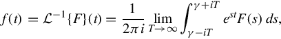
where γ is a real number so that the contour path of integration is in the region of convergence of F(s). An alternative formula for the inverse Laplace transform is given by Post’s inversion formula. In practice, it is typically more convenient to decompose a Laplace transform into the known transforms of functions obtained from a table, and construct the inverse by inspection.