Generalized inverse of matrix and solution of linear system equation
Abstract
This chapter presents a brief introduction to the generalized inverse of matrix, which is needed in the following expositions. This introduction includes the left inverse and right inverse, the Moore-Penrose inverse, the minimization approach to solve an algebraic matrix equation, the full rank decomposition theorem, the least square solution to an algebraic matrix equation, and the singular value decomposition.
Keywords
Generalized inverse of matrix; Left inverse; Right inverse; Moore-Penrose inverse; Full rank decomposition theorem; Least square solution to an algebraic matrix equation; Singular value decomposition
In this chapter, we briefly present some background for generalized inverse of matrix and its relation to solution of linear system equation, that is needed in the sequel. This chapter can be skimmed very quickly and used mainly as a quick reference. There have been a huge number of reference resources for this topic, to mention a few [43, 44, 51–54].
3.1 The generalized inverse of matrix
Recall how we defined the matrix inverse. A matrix inverse A−1 is defined as a matrix that produces identity matrix when we multiply with the original matrix A, that is, we define AA−1 = I = A−1A. Matrix inverse exists only for square matrices.
Real world data are not always square. Furthermore, real world data are not always consistent and might contain many repetitions. To deal with real world data, generalized inverse for rectangular matrix is needed.
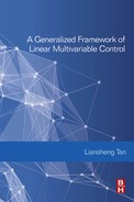
Generalized inverse matrix is defined as AA−A = A. Notice that the usual matrix inverse is covered by this definition because AA−1A = A. We use the term “generalized” inverse for a general rectangular matrix and to distinguish it from the inverse matrix that is for a square matrix. Generalized inverse is also called the pseudo-inverse.
Unfortunately there are many types of generalized inverse. Most generalized inverses are not unique. Some generalized inverses are reflexive satisfying (A−)− = A and some are not reflexive. In this tutorial, we will only discuss a few of them that are often used in practical applications.
• A reflexive generalized inverse is defined as
• A minimum norm generalized inverse, such that x = A−b will minimize ∥x∥ is defined as

• A generalized inverse that produces the least square solution that will minimize the residual or error ![]() , is defined as
, is defined as

3.1.1 The left inverse and right inverse
The usual matrix inverse is defined as a two-side inverse, i.e., AA−1 = I = A−1A because we can multiply the inverse matrix from the left or from the right of matrix A and we still get the identity matrix. This property is only true for a square matrix A.
For a rectangular matrix A, we may have a generalized left inverse or left inverse for short when we multiply the inverse from the left to get identity matrix Aleft−1A = I. Similarly, we may have a generalized right inverse, or right inverse for short, when we multiply the inverse from the right to get the identity matrix AAright = I.
In general, the left inverse is not equal to the right inverse. The generalized inverse of a rectangular matrix is related to the solving of system linear equations Ax = b. The solution to a normal equation is x = (ATA)−1ATb, which is equal to x = A−b. The term
is often called as generalized left inverse. Yet another pseudo-inverse can also be obtained by multiplying the transpose matrix from the right and this is called a generalized right inverse
3.1.2 Moore-Penrose inverse
It is possible to obtain a unique generalized matrix. To distinguish the unique generalized inverse from other nonunique generalized inverses A−, we use the symbol A+. The unique generalized inverse is called the Moore-Penrose inverse. It is defined using the following four conditions:
(2) A+AA+ = A+,
(3) (AA+)T = AA+,
(4) (A+A)T = A+A.
The first condition AA+A = A is the definition of a generalized inverse. Together with the first condition, the second condition indicates the generalized inverse is reflexive (A−)− = A. Together with the first condition, the third condition indicates that the generalized inverse is the least square solution that will minimize the norm of error ![]() The fourth condition above demonstrates the unique generalized inverse.
The fourth condition above demonstrates the unique generalized inverse.
Properties of generalized inverse of matrix: Some important properties of generalized inverse of matrix are:
1. The transpose of the left inverse of A is the right inverse Aright−1 = (Aleft−1)T. Similarly, the transpose of the right inverse of A is the left inverse Aleft−1 = (Aright−1)T.
2. A matrix Am×n has a left inverse Aleft−1 if and only if its rank equals its number of columns and the number of rows is more than the number of columns ρ(A) = n < m. In this case A+A = Aleft−1A = I.
3. A matrix Am×n has a right inverse Aright−1 if and only if its rank equals its number of rows and the number of rows is less than the number of columns ρ(A) = m < n. In this case A+A = AAright−1 = I.
4. The Moore-Penrose inverse is equal to left inverse A+ = Aleft−1, when ρ(A) = n < m and equals the right inverse A+ = Aright−1, when ρ(A) = m < n. The Moore-Penrose inverse is equal to the matrix inverse A+ = A−1, when ρ(A) = m = n.
3.1.3 The minimization approach to solve an algebraic matrix equation
The generalized inverse of the matrix has been used extensively in the areas of modern control, least square estimation and aircraft structural analysis. It is the purpose of this note to extend the results by presenting a unified framework that provides geometric insight and highlights certain optimal features imbedded in the generalized inverse.
Consider the algebraic matrix equation
where A is an n × m constant matrix, y is a given n vector, and x is an m vector to be determined. For the trivial case where n = m and A is a nonsingular matrix, i.e., rank(A) = n, a unique solution to Eq. (3.1) exists and is given by
where A−1 denotes the inverse of A.
For the case n≠m, the expression of x in terms of y involves the generalized inverse of A, denoted A+, and thus
In the following cases it will be shown that A+, for either n > m or n < m, may be viewed as a solution to a certain minimization problem.
With no loss of generality it can be assumed that A is of full rank, i.e.,
however, rank (A) < n. It is possible to delete the dependent columns of A, set the respective unknown components of x equal to zero, and reduce the problem to the case in which Eq. (3.4) is satisfied. Since the m columns of A do not span the n dimensional space Rn, an exact solution to Eq. (3.1) cannot be obtained if y is not contained in the subspace spanned by the columns of A. Thus, one is motivated to seek approximate solutions, the best of which is the one that minimizes the Euclidian norm of the error. Let the error e be given by
Then let z be given by
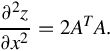
where the superscript “T” denotes the transpose. Evaluation of the gradient of z with respect to x yields
The Hessian matrix is
From Eq. (3.7), x is given by
By virtue of A having full rank, (ATA) is a positive definite matrix. Thus (ATA)−1 exists and the Hessian matrix is positive definite, implying that a minimum was obtained. In this case (n > m) the generalized inverse of A is given by
It is interesting to note that if y is contained in the subspace spanned by the columns of A, Eq. (3.9) yields an exact solution to Eq. (3.1), i.e., ∥e∥ = 0. The optimal feature of Eq. (3.9) has found extensive applications in data processing for least square approximations. In closing it should be noted that Eq. (3.9) can be obtained by invoking the Orthogonal Projection Lemma, thus providing a geometric interpretation to the optimal feature of Eq. (3.10).
Again, without loss of generality, it can be assumed that A is of full rank, i.e.,
If, however, rank(A) < n, it implies that some of the equations are merely a linear combination of the others and therefore may be deleted without loss of information, thereby reducing the case rank(A) < n to the case rank(A) = n. Moreover, if A is a square singular matrix, it can be reduced to case B after proper deletion of the dependent rows of A.
Eqs. (3.1), (3.11) with n < m yield an infinite number of solutions, the “optimal” of which is the one having the smallest norm. Therefore one is confronted with a constrained minimization problem, where the minimization of ∥x∥ (or equivalently ![]() ) is to be accomplished subject to Eq. (3.1). Adjoining the constraint, via a vector of Lagrange multipliers (λ), the objective function to be minimized is
) is to be accomplished subject to Eq. (3.1). Adjoining the constraint, via a vector of Lagrange multipliers (λ), the objective function to be minimized is
By evaluating the respective gradients
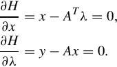
From Eq. (3.13), one has
Substitution of Eq. (3.15) into Eq. (3.14) yields
That is
The existence of (AAT)−1 is guaranteed by virtue of Eq. (3.11). Substitution of Eq. (3.17) into Eq. (3.15) yields
In this case (n < m) the generalized inverse of A is given by
For the sake of completeness it should be noted that the norm minimization of ∥e∥ and ∥x∥ of Eqs. (3.6), (3.12), respectively, can be performed by the extended vector norms, where a norm of a vector w is defined as wTQw and Q is a compatible positive definite weighting matrix. By doing so, one can choose the relative emphasis of the magnitudes of the vector components that is minimized.
For case A, Eq. (3.6) becomes
with the solution
From case B, Eq. (3.12) becomes
with the solution
In summary, a unified framework has been presented showing that the generalized inverse of a matrix can be viewed as a result of a minimization problem leading to a practical interpretation.
3.2 The full rank decomposition theorem
Concerning the situations of whether a matrix being full row rank or full column rank, we have the following obvious statement.
It is obvious that if A is of full row rank, then m ≤ n and if A is of full column rank, then m ≥ n. A sufficient and necessary condition for a matrix to be of full rank is that it is both of full row rank and of full column rank.
Theorem 3.2.2
Assuming A ∈ Cm×n, if there is a full column rank matrix F and full row rank matrix G making that
then A has a full rank decomposition.
Proof
For the matrix A, if rank A = r > 0, one is able to choose r linear independent columns from the columns of A: ![]() . The remaining columns can been expressed by these columns. That is, we have
. The remaining columns can been expressed by these columns. That is, we have
It is seen that, the matrix F is a full column rank matrix. Therefore, there exists permutation matrix Q and S such that
Letting G = [IrS]Q−1, G is a full row rank matrix. So A has a full rank decomposition
Proof
If λ is any eigenvalue of FHF, the vector x is the corresponding nonzero feature vector, one has
In this case, we have
Considering F is a full column rank matrix, and Fx≠0, so ![]() . We therefore draw the conclusion: λ > 0.
. We therefore draw the conclusion: λ > 0.
Analogously, if G ∈ Cr×n is a full row rank matrix, then GGH has the above properties. When A ∈ Cm×n, B ∈ Cn×m, if AB = Im, then B is the right inverse of A denoted by B = Aright−1 and A is the left inverse of B denoted by A = Bleft−1.
3.3 The least square solution to an algebraic matrix equation
The method of least squares is a standard approach in regression analysis to the approximate solution of the over determined systems, in which among the set of equations there are more equations than unknowns. The term “least squares” refers to this situation, the overall solution minimizes the summation of the squares of the errors, which are brought by the results of every single equation.
3.3.1 The solution to the compatible linear equations
We have the following general solution of a given linear matrix equation, which is formulated in terms of the Moore-Penrose inverse.
Theorem 3.3.1
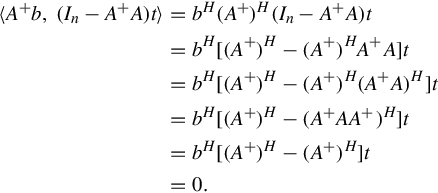
If A ∈ Cm×n, b ∈ Cm, x ∈ Cn, and if the system of linear equations Ax = b is compatible, the general solution is given by
Proof
Because Ax = b is compatible, there is a x0 making Ax0 = b. So we have on one hand
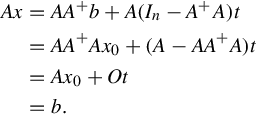
On the other hand, if x0 is any solution of Ax = b, such that t = x0. Therefore,
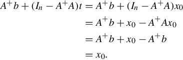
So far, we have proved that
is the general solution of the equation Ax = b, which concludes the proof.
In particular, when b = 0, we obtain the general solution of the homogeneous linear equations Ax = 0 given by
3.3.2 The least square solution of incompatible equation
Considering in many applications, such as data processing, multivariate analysis, optimization theory, modern control theory, and networking theory, the mathematical model of linear matrix equation is often an incompatible one. We hereafter use the generalized inverse matrix to represent the following general solution of incompatible linear equations.
Theorem 3.3.2
When A ∈ Cm×n, b ∈ Cm, if there is x*∈ Cn such that
then the component x* is termed as the least square solutions to the system of equations Ax = b.
Theorem 3.3.3
When A ∈ Cm×n, all the least square solutions of system of equation Ax = b are given by
Proof
∀x ∈ Cn, we define
and denote x = μ + iν (μ, ν ∈ Rn), we then have
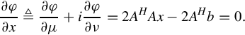
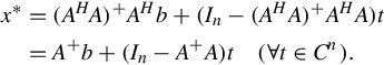
Therefore we have AHAx = AHb. Because
due to the rank of the augmented matrix is equal to that of the coefficient matrix, so AHAx = AHb is compatibility equations. Assuming φ(x) is nonnegative real function, according to multivariate function extreme value theory, the solution of normal equations is the minimum point of φ(x). Subsequently, the total least square solution of equations Ax = b is
3.3.3 The minimum norm least squares solution for the equations
From the above discussions, whether the equations are compatible or not, the least-square solutions can be expressed as
Because the least squares solution is not unique, one is able to find a least square solution of minimum norm, which is given by
where x** is referred to as the very minimal norm least square solution to the equations Ax = b. We have the following theorem:
3.4 The singular value decomposition
The Moore-Penrose inverse can be obtained through singular value decomposition (SVD): A = UDVT, such that A+ = V D−1UT. We have the following definition
Definition 3.4.1
When A ∈ Cm×n, denote the following positive characteristic values for Hermite matrix AHA
Then
are the single values of A.
If A ∈ Cm×n, rank A = r, then AHA has r positive eigenvalues and the remaining eigenvalues are zeros. Further, we assume that they can be ordered in the following manner
Theorem 3.4.1
When A ∈ Cm×n, rank A = r > 0, the so-called singular value decomposition (SVD) of A is
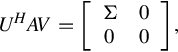
where the matrix U is the m order unitary matrix, the matrix V is the n order unitary matrix, and the matrix Σ is the following diagonal matrix
Note in the above the component r is the positive singular value of A.
Proof
If ![]() are all the eigenvalues of A, and σ1 ≥ σ2 ≥⋯ ≥ σr > 0. Because AHA is nonnegative definite Hermite matrix, there is a unitary matrix V with the order n, satisfying the following associations
are all the eigenvalues of A, and σ1 ≥ σ2 ≥⋯ ≥ σr > 0. Because AHA is nonnegative definite Hermite matrix, there is a unitary matrix V with the order n, satisfying the following associations

Among them ![]() . By partitioning the matrix V into some subblocks
. By partitioning the matrix V into some subblocks
then we will have
Then
So
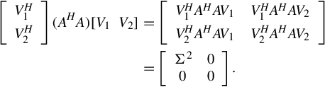
By letting
where U1 is part of the unitary matrix and extending it into an m order unitary matrix U = [U1U2], U2 is part of the column unitary matrix, we thus have
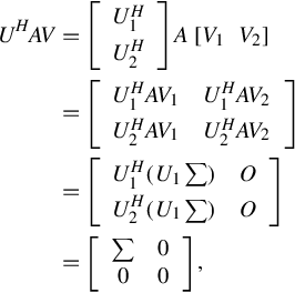
which concludes the proof.
Singular value decomposition is a factorization of a rectangular matrix A into three matrices U, D, and V. The two matrices U and V are orthogonal matrices (UT = U−1, V VT = I) while D is a diagonal matrix. The factorization means that we can multiply the three matrices to get back the original matrix A = UDVT. The transpose matrix is obtained through AT = V DUT. Since both orthogonal matrix and diagonal matrix have many nice properties, SVD is one of the most powerful matrix decomposition and is used in many applications, such as the least square solution (regression), feature selection (PCA, MDS), spectral clustering, image restoration and three-dimensional computer vision (fundamental matrix estimation), equilibrium of Markov Chain, and many others.
Matrix U and V are not unique, their columns come from the concatenation of eigenvectors of symmetric matrices AAT and ATA. Since eigenvectors of symmetric matrix are orthogonal (and linearly independent), they can be used as basis vectors (coordinate system) to span a multidimensional space. The absolute value of the determinant of orthogonal matrix is one, thus the matrix always has inverse. Furthermore, each column (and each row) of orthogonal matrix has unit norm. The diagonal matrix D contains the square of eigenvalues of symmetric matrix ATA. The diagonal elements are nonnegative numbers and they are called singular values. Because they come from a symmetric matrix, the eigenvalues (and the eigenvectors) are all real numbers (no complex numbers).
Numerical computation of SVD is stable in terms of round off error. When some of the singular values are nearly zero, we can truncate them as zero and it yields numerical stability. If the SVD factor matrix A = UDVT, then the diagonal matrix can also be obtained from D = UTAV. The eigenvectors represent many solutions of the homogeneous equation. They are not unique and correct up to a scalar multiple.
Properties: SVD can reveal many things:
1. Singular value gives valuable information as to whether a square matrix A is singular. A square matrix A is nonsingular (i.e., have inverse) if and only if all its singular values are different from zero.
2. If the square matrix A is nonsingular, the inverse matrix can be obtained by
3. The number of nonzero singular values is equal to the rank of any rectangular matrix. In fact, SVD is a robust technique to compute matrix rank against ill-conditioned matrices.
4. The ratio between the largest and the smallest singular value is called the condition number, which measures the degree of singularity and reveals ill-conditioned matrix.
5. SVD can produce one of matrix norms, which is called the Frobenius norm, by taking the sum of square of singular values
The Frobenius norm is computed by taking the sums of the square elements in the matrix.
6. SVD can also produce a generalized inverse (pseudo-inverse) for any rectangular matrix. In fact, the generalized inverse is also a Moore-Penrose inverse by setting
where the matrix ![]() is equal to D−1 but all nearly zero values are set to zero.
is equal to D−1 but all nearly zero values are set to zero.
7. SVD also approximates the solution of the nonhomogenous linear system AX = b such that the norm is minimum ![]() . This is the basic of least square, orthogonal projection and regression analysis.
. This is the basic of least square, orthogonal projection and regression analysis.
8. SVD also solves the homogenous linear system by taking the column of VT, which represents the eigenvector corresponding to the zero eigenvalue of symmetric matrix ATA.