
Internet congestion control
A linear multivariable control look
Abstract
The working mechanism of today’s Internet is a feedback system, which has the responsibilities of managing the allocation of bandwidth resources among competing traffic flows and controlling the congestion. Congestion control mechanisms in the Internet represent some of the largest deployed artificial feedback systems. The main aim of this chapter is to give an outline for the Internet congestion control from the perspective of a linear multivariable control system. We bring this subject into a control domain by looking at and those between the dynamics of individual flow rates and the dynamics of aggregate flow rates, the transferring relations between link price and flow aggregate price from a multivariable control point of views including the Smith-McMillan forms. Finally we look at the issue of feedback control design to relate the transport control protocol (TCP) source flow rate with the aggregate flow price which is in a proportional (P) controller structure. These analyses of the flow level then constitute a theoretical basis for TCP protocol design in the packet level.
Keywords
Internet; Congestion control; Flow dynamics; Primal-dual algorithm; Linear multivariable control system; Smith-McMillan form; Proportional (P) controller; Transmission control protocol; Active queue management; Feedback; ACK; Packet level; Flow level; Stability
Congestion control mechanisms in the Internet represent one of the largest deployed artificial feedback systems.
(from [42])
The working mechanism of today’s Internet is a feedback system, which has the responsibilities of managing the allocation of bandwidth resources among competing traffic flows and controlling the congestion. Being sharply different from the traditional telephony network, where resources are allocated by the network core using an admission policy, the Internet’s resources are allocated in a real-time manner, mainly by the end computer and communication systems themselves. The response is required to meet the desire to accommodate a diversity of demands, from “mice” being made of a few packets, to long “elephants” being greedy for whatever bandwidth is available, and to avoid a centralized allocation mechanism while performing all the manipulations in a distributed manner. The fact that end-systems must control their throughput with little information about the overall network facilitates the use of feedback; such mechanisms have been incorporated since the late 1980s [129] (the well-known Jacobson’s congestion avoidance algorithm) into the transport control protocol (TCP) layer of the Internet protocol (IP) stack. For a survey of these algorithms, see [42].
Congestion control and resource allocation mechanisms in today’s wireless and wire-lined networks, including the Internet, have already represented many challenges in design, as they continues to expand in size, diversity, reaching scope, integration, and convergence. Having a deep understanding of how their fundamental resource is controlled, and how the allocated resource is contributing to congestion control and service quality, becomes extremely important. Computer networks including the Internet are initially designed on a heuristic, intricate basis of many control mechanisms microscopically on the packet level, they are understood afterwards macroscopically in the flow level.
The notable approaches to address the congestion control and resource allocation issues from a macroscopic perspective are the primal algorithm, the dual algorithm, and the primal-dual algorithm. All these algorithms result from the network utility maximization model. The significance in these algorithms are in terms of the modeling of the congestion measuring and source actions, which is presented in the following:
• Links can feedback to data sources information on the congestion in the resources being used. It is assumed that each network link measures its congestion by a scalar variable (termed price) and that sources have information on the aggregate price of links in their path.
• After gaining congestion information, flows can take action by using their control mechanisms to react to the congestion along the path to adjust their sending rate.
These assumptions are implicitly presented in many variants of today’s TCP protocols. The price signal being used in these protocols can be, for example, loss probability and queueing delay. Also, it is the natural setting for exploring alternative protocols based on more explicit price signaling; for example, the random marking and random dropping actions of packet.
In the primal-dual congestion control algorithm, there are two key blocks: the source rates are adjusted to be adapted to aggregate prices in the TCP algorithm and the link prices are updated in terms of link utilization. Mathematically, we can model the TCP/AQM systems by the following general forms:
The first equation in the above is the mechanism of source rate vector X updating in terms of the aggregate price vector Q, while the second equation in the above is responsible for generating the link price vector P in terms of the aggregate flow rate Y. Note that F(X(t), Q(t)) and G(P(t), Y (t)) are matrix functions, which are involved into generating the source rate vector and the link price vector. Being deviated from the model presented by Low et al. [42] and Wang [130], herein we are considering a more general communication model, where there are possibly multicast communications.
A multicast (one-to-many or many-to-many distribution [131]) is group communication, where information is addressed to a group of destination computers simultaneously. Group communication has two forms: application layer multicast and network assisted multicast. The network assisted multicast makes it possible for the source to efficiently send to a specific group in a single transmission. Copies are automatically created in other network elements, such as routers, switches, and cellular network base stations, but only to network segments that currently contain members of the group. One typical example of multicast communications is the IP multicast. IP multicast is a technique for one-to-many communication over an IP infrastructure in a network. The destination nodes send join and leave messages, for example in the case of Internet television when the user changes from one TV channel to another. IP multicast scales to a larger receiver population by not requiring prior knowledge of the identity of number of receivers. Multicast uses network infrastructure efficiently by requiring that the source send a packet only once, even if it needs to be delivered to a large number of receivers. The nodes in the network take care of replicating the packet to reach multiple receivers only when it is necessary.
In the situation of multicast, there are interactions (coupled components) in the source rate vector X and in the link price vector P, as one source may issue more than one flow and the link may set more than one price value for a flow. In the usual model presented in, for example, [42, 130], an inherited assumption is that any source only issues one flow. This usual model does not consider the multicast flows and multiple pricing mechanism. Therefore in our model presented in Eqs. (15.1), (15.2) there may be interactions among the components of X and P. This is the reason why we have written the source rate updating and the link price updating mechanisms into the matrix equation forms rather than the individual and independent equations as in Eqs. (15.1), (15.2).
The complete system, which is coupled and interacted by Eqs. (15.1), (15.2), determines both the equilibrium and dynamic characteristics of the TCP/AQM network [130]. However, the equilibrium point is not necessarily unique and it will depend on the initial settings of the system. Therefore the dynamic characteristics of the network may have a diversity. This issue is, however, very complex and deserves further study.
The mechanism of the source rate updating and link price updating, the relation between the individual source rate and link aggregate rate, which is related to the routing matrix, and the relation between the individual link price and the aggregated flow price, which is also related to the routing matrix, are demonstrated in Fig. 15.1.
As a distributed algorithm [132] to allocate network resources among competing users, congestion control consists of two components: a source algorithm that dynamically adjusts the rate in response to the congestion in its path, and a link algorithm that implicitly or explicitly, updates a congestion measure and sends it back to the sources that use that link. In the current Internet, the source algorithm is carried out by TCP, and the link algorithm by active queue management (AQM) schemes. The TCP algorithms include TCP Reno [129], TCP Vegas [133, 134], High-speed TCP [135], Scalable-TCP [136], FAST TCP [137–139], and Generalized FAST TCP [132, 140]; while the AQM algorithms include Drop-Tail [141], RED [142], BLUE [143], REM/PI [144], and AVQ [139, 145]. The working mechanism of the TCP algorithms and the AQM algorithms in the Internet are displayed in Fig. 15.2.

Different protocols use different metrics to measure congestion. For example, TCP Reno [129] and its variants use loss probability as congestion measure, while TCP Vegas [133, 134], FAST TCP [137, 139], and the generalized Fast TCP [140] use queueing delay.
It is established in [146, 147] that, the overall operations of TCP congestion control algorithms work very similarly to a time-delayed closed-loop control system. The feedback control theory for time-delayed systems have been successfully used to enhance the performance of the TCP/RED system in a very logical manner in [146, 147]. Other developments on stability of TCP/AQM systems along the line of control theory can be found in [148–153].
The main aim of this chapter is to give an outline of the Internet congestion control from the perspective of linear multivariable control system. We bring this subject into a control domain by looking at the transferring relations between the dynamics of individual flow rates and the dynamics of aggregate flow rates, the transferring relations between link price and flow aggregate price from a multivariable control point of views including the Smith-McMillan forms. Finally, we look at the issue of feedback control design to relate the TCP source flow rate with the aggregate flow price, which is in a proportional (P) controller structure. These analyses in the flow level then constitute a theoretical basis for TCP protocol design on the packet level.
15.1 The basic model of Internet congestion control
This section presents the basic model of Internet congestion control.
Consider a network that consists of a set L = {1, …, M} of unidirectional links of capacity cl, l ∈ L. The network is shared by a set I = {1, …, N} of sources. Let xi be the rate of flow i and let X(t) = {xi(t), i ∈ I} be the rate vector. Let R = (Rli, i ∈ I, l ∈ L) be the routing matrix, where Rli = 1 if flow i traverses link l, and 0 otherwise. By introducing the link rate vector Y (t) = {yl(t), l ∈ L}, the link price vector P(t) = {pl(t), l ∈ L}, and the source price vector Q(t) = {qi(t), i ∈ I}, we then have
It is noted that the above two equations relate the individual source rate vector with the aggregate flow (at the links) rate vector and the individual link price vector with the source aggregate price vector.
At time t, we assume link l observes the aggregate source rate

and source i observes the aggregate price in its path
where ![]() is the forward feedback delay from source i to link l, and
is the forward feedback delay from source i to link l, and ![]() is the backward feedback delay from link l to source i. For simplicity, we assume that the feedback delays
is the backward feedback delay from link l to source i. For simplicity, we assume that the feedback delays ![]() and
and ![]() are constants. Further, we consider propagation delay and neglect the queueing delay, thus treating round trip delay for any link l on the path of source i, i.e.,
are constants. Further, we consider propagation delay and neglect the queueing delay, thus treating round trip delay for any link l on the path of source i, i.e., ![]() , as a constant.
, as a constant.
15.2 Internet congestion control: A multivariable control look
In this section, by describing the congestion control network model as a time-delayed multivariable control system, we propose a method to analyze the transfer functions between the individual source rate and the link aggregate rate, between the link price and the source aggregate price. Based on this, we look at the issue of feedback control design to relate the TCP source flow rate with the aggregate flow price, which is in a proportional (P) controller structure. This can further be utilized to analyze the important properties, such as stability, of the network systems.
Stability of the algorithm in Internet congestion control is especially important when it is implemented within a network. For example, to have an efficient throughput, to bound the delay and to minimize packet loss, the rate of data flow through its links should tend toward an equilibrium value, rather than continually oscillating between having bandwidth spare and being completely overloaded. Given the fact that the control system structure of Eqs. (15.5), (15.6) like the Smith-McMillan form governs their system performance, e.g., the stability, let us take a closer look.
Taking the Laplace transform of Eqs. (15.5), (15.6), respectively, and writing the delay routing matrices in the frequency domain as
where
and
where

we then have
where X(s), Y (s), P(s), and Q(s) denote the Laplace transform of the vectors X(t), Y (t), P(t), and Q(t), respectively, and T denotes the transport of the matrix.
15.3 Padé approximations to the system (15.7) and (15.8)
Polynomials are not such a good class of functions if one wants to approximate functions with singularities because polynomials are entire functions without singularities. They are only useful up to the first singularity. Rational functions are the simplest ones with singularities. The idea is that the poles of the rational functions will move to the singularities of the function and hence the domain of convergence can be enlarged, and singularities of it may be discovered using the poles of the rational approximations.
The [m, n] Padé approximation of a function f in a point a is the rational function ![]() with Qm a polynomial of degree ≤ m and Pn a polynomial of degree ≤ n, for which we have the following interpolation condition at a
with Qm a polynomial of degree ≤ m and Pn a polynomial of degree ≤ n, for which we have the following interpolation condition at a
The computation of the polynomials Pn and Qm is not so straightforward in the above condition since one first has to compute the Taylor expansion of ![]() and then equate the first m + n + 1 Taylor coefficients to the first m + n + 1 Taylor coefficients of f. Usually the Padé approximation is defined by linearizing the interpolation condition as
and then equate the first m + n + 1 Taylor coefficients to the first m + n + 1 Taylor coefficients of f. Usually the Padé approximation is defined by linearizing the interpolation condition as
For Padé approximation near infinity to a function of the form

we let m = n − 1 and the interpolation condition is
There is a degree of freedom since we can multiply both sides of Eq. (15.10) by a constant. Usually we normalize this by taking Pn monic, that is it is in the form xn + ⋯, when this is possible. This can only be done if Pn is of the exact degree n. If we take Pn monic, then we can determine the n unknown coefficients ak (k = 1, …, n) in
by putting the coefficients of (z−a)k for k = m + 1, m + 2, …, m + n in the Taylor expansion of Pnf equal to zero. The polynomial Qm then corresponds to the Taylor polynomial of degree m of Pnf.
Hereafter we present another approach. Suppose f is analytic in a domain Ω that contains a. Again we take a contour Γ inside Ω encircling a once in the positive direction. Divide both sides of Eq. (15.10) by (z−a)m+k+2 and integrate, to find
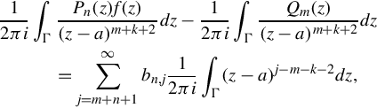
where the bn, js are the coefficients in the expansion of Pnf − Qm around a. The integral involving Qm is zero for k ≥ 0 since it is proportional to the (m + k + 1)th derivative of Qm, which is zero for k ≥ 0. The summation on the right-hand side has a contribution only when j = m + k + 1, but when 0 ≤ k ≤ n − 1 then j ≤ m + n, and such indices do not appear in the summation. Hence the right hand side also vanishes for k ≤ n − 1. Therefore Eq. (15.10) tells us that
If we use the expansion (15.11) then this gives

and then

Therefore we obtain the following system of equations
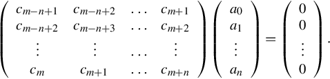
There is one degree of freedom here since we have n + 1 unknowns and n (homogeneous) equations. The choice a0 = 1 (if possible) gives the monic polynomial Pn, but sometimes other normalization will be used.
15.3.1 Padé approximation to the transfer functions of the time-delay system (15.7) and (15.8)
For the transfer function of a time-delay system
which is irrational (it has no s-polynomial in the numerator and in the denominator), in some situations as in analyzing the frequency response of this sort of control system containing a time-delay, it is necessary to substitute e−τs with the following Padé approximation
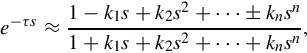
where n is the order of the approximation.
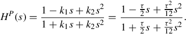
In particular, to find a second order Padé approximation (n = 2) for the time-delay transfer function H(s), we have
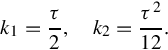
Subsequently, the second order Padé approximation to the transfer function H(s), denoted by HP(s), comes out to be
With regard to the Padé approximation to the time-delay system (15.7) and (15.8), so far we are able to establish the following result.
Theorem 15.3.1
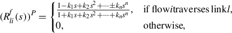
The Padé approximations to the time-delay system (15.7) and (15.8) are given by
where ![]() and
and ![]() are the respectively Padé approximations to the transfer function matrices (with delays) Rf(s) and (Rb(s))T. They are given by
are the respectively Padé approximations to the transfer function matrices (with delays) Rf(s) and (Rb(s))T. They are given by
where
and
where
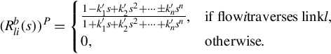
In the above, all the parameters ki (i = 1, 2, …, n) and ki′ (i = 1, 2, …, n) can be determined with relations to the order of the approximation and the delays.
It should be noted that the above theorem is very important for us to explore the system structure of Internet congestion control, in that it has actually reduced the original transfer functions from irrational to rational. This enables us to work on the rational function matrices given in Eqs. (15.16), (15.17) by using the generalized linear multivariable control approaches.
15.3.2 A proportional controller
Now we design the following proportional control to relate the source rate with the experienced aggregate price of that source
where 0 ≤ ψi ≤ 1 is the control gain.
We have the following formulations to calculate the congestion price. For a given flow that traverses a set of link Li, if all the packet loss probabilities pl(t) at all links are small enough, the end-to-end packet loss probabilities qi(t) satisfy
The aggregate queuing delay for that flow is given by
where bl is the backlog at link l and cl is the leaking capacity of the link.
From a TCP protocol point of view, the controller (15.18) suggests that if qi represents congestion price (either queuing delay or packet loss probability) in the sources path, the source rate should be a monotonically decreasing function of it. Specifically, as a larger queuing delay or packet loss probability suggests a higher degree of congestion, the source rate should be decreased proportionally to the congestion degree parameter (the aggregate queuing delay or the aggregate packet loss probability). Alternatively, if a source is likely to experience slight congestion along its path, i.e., the aggregate queuing delay or the aggregate packet loss probability is smaller, one should increase the sending rate for this source.
Combining all the above N equations (15.18) together, we have the following matrix equation
where Ψ = diag{ψ1, ψ2, …, ψN}. By taking the Laplace transform of the above equation and then substituting this Laplace transformed form into Eq. (15.16), with Eq. (15.17) being considered, we arrive at the following relation between Y (s) and P(s)
The above equation is the Padé approximation to the transfer function from the link price vector to the link aggregate rate vector. We will work on it to gain insights into its frequency structure later on by using a simple network example.
15.4 Analyses into system structure of congestion control of a simple network in frequency domain
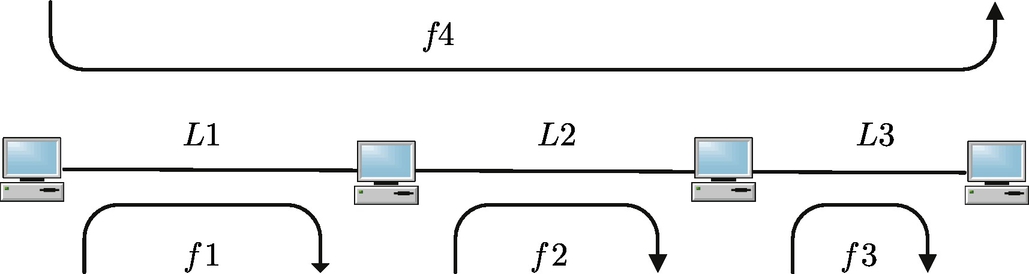
Let us consider a simple network with three links and four flows as shown in Fig. 15.3. In this network, there are four flows: f1 traverses link L1, f2 traverses link L2, f3 traverses link L3, and f4 traverses link L1, link L2, and link L3. Flows f1, f2, and f3 represent one-hop short flow, which is dominant in the Internet: most peer-to-peer applications involve one-link flows between a data source and a receiver (downloader); while flow f4 represents long flows which traverse more than one hop. The routing structure of this network is described by the following routing matrix

Letting xi denote the source sending rate of flow fi, (i = 1, 2, 3, 4). The individual flow rate vector is then

Letting yl (l = 1, 2, 3) denote the aggregate flow rate at link l, the aggregate flow rate vector is then denoted by
Each link is suggesting a price (either delay or packet loss ratio), one has the link price vector
The total price for flow fi is the sum of all the prices for all links it traverses and is denoted by qi. We then denote the aggregate price vector as
The aggregate flow rate vector and the individual rate vector is associated by the routing matrix, and the aggregate price vector and the individual price vector are also associated by the transpose of the routing matrix. They are mathematically described by
In particular, at time t, the links observe the following corresponding aggregate source rate
where ![]() (l = 1, 2, 3;i = 1, 2, 3, 4) denotes the feed-forward delay of the data flow fi by the traveling link l. This delay is determined by the propagation delay and the forward queuing delay at the link. The propagation delay is determined by the distance between the source and the destination while the forward queuing delay is determined by the queue length and the leaking capacity at the link.
(l = 1, 2, 3;i = 1, 2, 3, 4) denotes the feed-forward delay of the data flow fi by the traveling link l. This delay is determined by the propagation delay and the forward queuing delay at the link. The propagation delay is determined by the distance between the source and the destination while the forward queuing delay is determined by the queue length and the leaking capacity at the link.
Similarly, the sources observe the following corresponding aggregate price along their path
where ![]() (l = 1, 2, 3;i = 1, 2, 3, 4) denotes the feed-backward delay of flow fi. These backward delays are actually experienced by the acknowledgment (ack) packets for their corresponding data flows. They are all related to the distance between the destination and the source and the capacity (in the opposite direction) correspondingly.
(l = 1, 2, 3;i = 1, 2, 3, 4) denotes the feed-backward delay of flow fi. These backward delays are actually experienced by the acknowledgment (ack) packets for their corresponding data flows. They are all related to the distance between the destination and the source and the capacity (in the opposite direction) correspondingly.
By taking the Laplace transform of Eqs. (15.23), (15.24), (15.25), and denoting the Laplace transformation of X(t) and Y (t) as X(s) and Y (s), respectively, one has
where the transfer function ![]() is given by
is given by
The second order Padé approximation to the above transfer function is
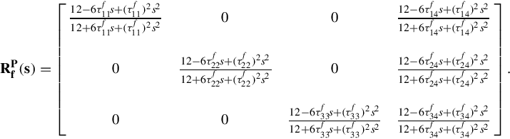
If we set all the forward delays as ![]() by denoting
by denoting

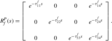
then we have the following approximated transfer function
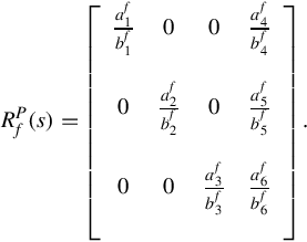
Using df(s) to denote the least common multiple (lcm) of the denominators of all the elements of ![]() , one has
, one has
Subsequently the Smith form of ![]() is Sf(s), which is given by
is Sf(s), which is given by

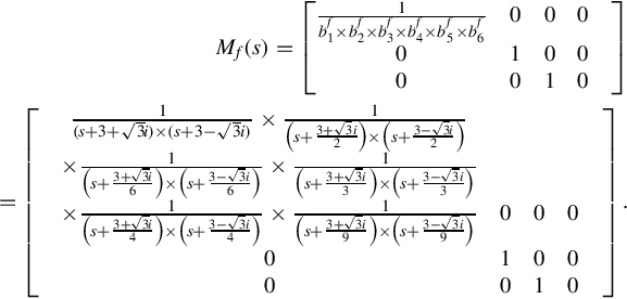
Accordingly the Smith-McMillan form of ![]() is Mf(s)
is Mf(s)
Similarly, by taking the Laplace transform of Eqs. (15.26), (15.27), (15.28), (15.29), and denoting the Laplace transformation of P(t) and Q(t) as P(s) and Q(s), respectively, one has
where the transfer function ![]() is given by
is given by

If the backward delays are set as ![]() by denoting
by denoting

we then have
Further, if db(s) is the least common multiple (lcm) of the denominators of all the elements in ![]() , that is
, that is
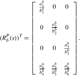
then the Smith form of ![]() (denoted by Sb(s)) is given by
(denoted by Sb(s)) is given by
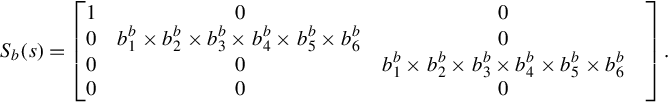
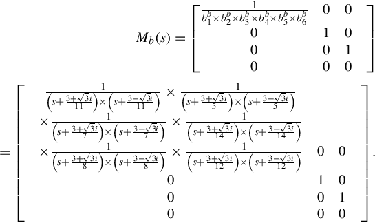
Therefore the Smith-McMillan form of ![]() (denoted by Mb(s)) is given by
(denoted by Mb(s)) is given by
Now we design the following proportional control to relate the source rate with the experienced aggregate price of that source
where 0 ≤ ψi ≤ 1 is the control gain. The transfer function from P(s) to Y (s) is then given by
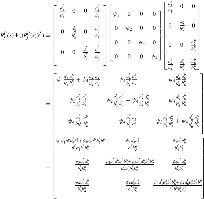
In the above all the elements are given by
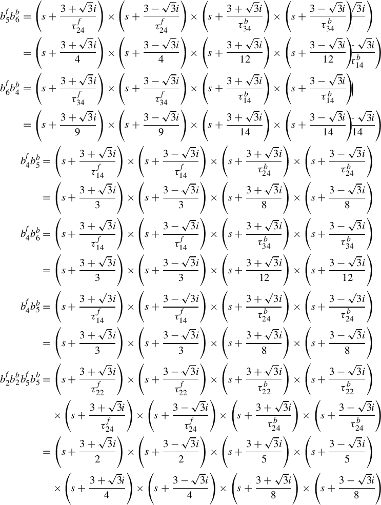
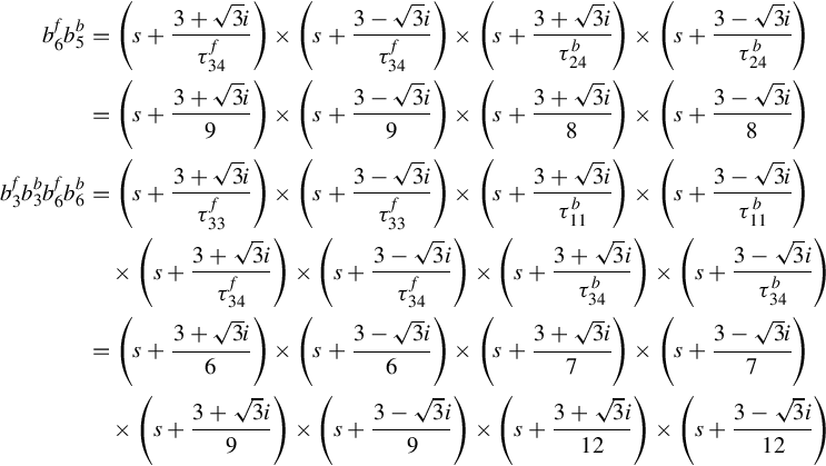
Therefore one finds that all the poles of the matrix ![]() are
are

Observing from the above analyses, one finds that all the poles of the open-loop transfer functions from X(s) to Y (s) and from P(s) to Q(s), and the closed-loop transfer function from P(s) to Y (s) are lying in the left half complex plane. This suggests that all the three considered systems are bounded-input bounded-output (BIBO) stable. However, note that we have taken the second-order Padé approximation. The stability of the systems may be specific to the particular Padé approximations.