A refined resolvent decomposition of a regular polynomial matrix and application to the solution of regular PMDs
Abstract
This chapter presents a resolvent decomposition which is a refinement of the state-of-the-art results. It is formulated in terms of the notions of the finite Jordan pairs, infinite Jordan pairs, and the generalized infinite Jordan pairs. We make clear the issue of infinite Jordan pair noted by a number of references. This refined resolvent decomposition captures the essential feature of the system structure. Further, the redundant information, which is included in the known resolvent decomposition, is deleted through a certain transformation, thus the resulting resolvent decomposition inherits the advantages of the reported results. This refined resolvent decomposition facilitates computation of the inverse matrix of A(s) due to the fact that the dimensions of the matrices used are of minimal.
Based on this proposed resolvent decomposition, a complete solution of a polynomial matrix description (PMD) follows that reflects the detailed structure of the zero state response and the zero input response of the system. The complete impulsive properties of the system are also displayed in our solution. Such impulsive properties are not completely displayed in the known solution. Although for the homogeneous case this problem is considered in the literatures, the complete impulsive properties of the system for the general nonhomogeneous regular PMD are not discussed. Our approach is stable in numerical computation terms, for it avoids an extraordinarily large number of polynomial manipulations.
Keywords
Resolvent decomposition; The finite Jordan pairs; Infinite Jordan pairs; The generalized infinite Jordan pairs; Polynomial matrix description; The zero state response; The zero input response
9.1 Introduction
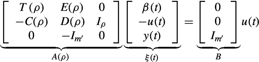
Regular polynomial matrix descriptions (PMDs) are described by

where ρ := d/dt is the differential operator,
![]() is the pseudo-state of
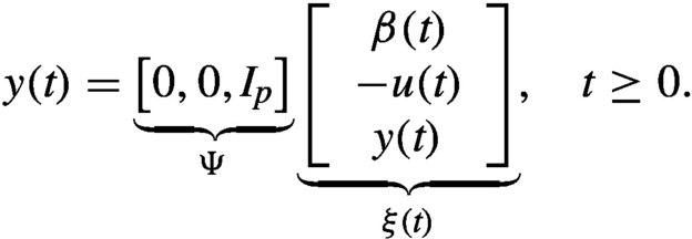
is the pseudo-state of ![]() is the control input and y(t) the output of Σ′. Σ′can be written in the form:
is the control input and y(t) the output of Σ′. Σ′can be written in the form:
In order to investigate the solution of the above PMD, we thus focus our interests on the following form of equation
where ![]() , with
, with ![]() . The homogeneous case of Σ is
. The homogeneous case of Σ is
Both regular generalized state space systems which are described by
where E is a singular matrix, rank(ρE − A) = r, and the (regular) state space systems which are described by
are special cases of the regular PMDs (Eq. 9.1).
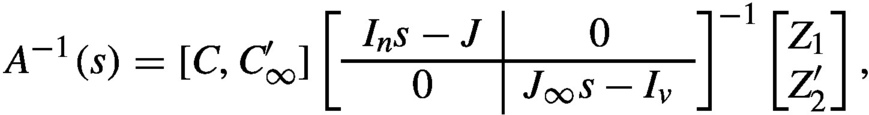
The solution of the above PMDs can be proposed on the basis of any resolvent decomposition of A(s) given by
where (C, J) is the finite Jordan pair of A(s), and ![]() is the infinite Jordan pair [13, 17] of A(s). Such resolvent decompositions are not unique, but play an important role in formulating the solution of regular PMDs. The difficulties in the problem of obtaining the solution of the PMD are specific to the particular resolvent decomposition used. From a computation point of view, when the matrices in Eq. (9.3) are of minimal dimensions, it is obviously easiest to obtain the inverse matrix of A(s).
is the infinite Jordan pair [13, 17] of A(s). Such resolvent decompositions are not unique, but play an important role in formulating the solution of regular PMDs. The difficulties in the problem of obtaining the solution of the PMD are specific to the particular resolvent decomposition used. From a computation point of view, when the matrices in Eq. (9.3) are of minimal dimensions, it is obviously easiest to obtain the inverse matrix of A(s).
There is fundamental interest (notably [13, 17, 102]) in the solution of the regular PMD and its homogeneous case. For Eq. (9.1) Gohberg et al. [17] proposed a particular resolvent decomposition, and the solution of it was formulated according to this decomposition. However, the impulsive property of the system at t = 0 was not properly considered in this work. One advantage of this resolvent Decomposition, however, is that it is constructive, due to the fact that the matrices ![]() in Eq. (9.3) are formulated in terms of the finite and infinite Jordan pairs. On the other hand in this resolvent decomposition, there appears to be certain redundant information, in that the dimensions of the infinite Jordan pair are much larger than is usually necessary, this in turn brings some inconvenience in computing the inverse matrix of A(s).
in Eq. (9.3) are formulated in terms of the finite and infinite Jordan pairs. On the other hand in this resolvent decomposition, there appears to be certain redundant information, in that the dimensions of the infinite Jordan pair are much larger than is usually necessary, this in turn brings some inconvenience in computing the inverse matrix of A(s).
In fact some of the infinite elementary divisors [18] that correspond to the infinite poles of A(s) actually contribute nothing to the solution, as will be seen subsequently. Thus a resolvent decomposition can be proposed in a simpler form that has the further advantage of giving a more precise insight into the system structure as well as bringing some convenience in actual computation. Vardulakis [13] obtained a general solution of Eq. (9.1) under the assumption that the initial conditions of ξ(t) are zero. The main idea of this approach is to find minimal realizations of the strictly proper part and the polynomial part of A−1(s) and then to obtain the required resolvent decomposition. Although this procedure does give good insight into the system structure, the realization approach is not so straightforward by itself and it is consequently more difficult to apply in actual computation. Furthermore, in this procedure, no explicit formula for Z and ![]() is available.
is available.
In [102] the solution and the impulsive behavior of autonomous linear multivariable systems whose pseudo-state obeys the linear matrix differential equation (9.2) are examined. The impulsive solution part of the general nonhomogeneous PMD (Eq. 9.1) is, however, not displayed in the solution of Eq. (9.2) given by Vardulakis et al. [102]. Apparently, differences arise between the solution of Gohberg et al. [17] and that of Vardulakis [13] due to the fact that these two solutions are expressed through two different resolvent decompositions. Although it is found that the redundant information contained in the solution of Gohberg et al. [17] decouples in the meaning described in this book, an overly large resolvent decomposition definitely brings some inconvenience to actual computation.
The main purpose of this chapter is to present a resolvent decomposition that is a refinement of both results obtained by Gohberg et al. [17] and Vardulakis [13]. It is formulated in terms of the notions of the finite Jordan pairs, infinite Jordan pairs, and the generalized infinite Jordan pairs that were defined by Gohberg et al. [17] and Vardulakis [13]. We clarify the issue of the infinite Jordan pair noted by Gohberg et al. [17] and Vardulakis [13]. This refined resolvent decomposition captures the essential feature of the system structure, and the redundant information that is included in the resolvent decomposition of Gohberg et al. [17] is deleted through certain transformations. The resulting resolvent decomposition thus inherits the advantages of both the results of Gohberg et al. [17] and that of Vardulakis [13].
Based on this proposed resolvent decomposition, a complete solution of a PMD follows that reflects the detailed structure of the zero state response and the zero input response of the system. The complete impulsive properties of the system are also displayed in our solution. Such impulsive properties are not properly displayed in the solution of Gohberg et al. [17]. Although for the homogeneous case it is considered in Vardulakis [13], Vardulakis et al. [102], such a complete treatment of the impulsive properties of the system for the general nonhomogeneous regular PMD is not available in Vardulakis [13] and Vardulakis et al. [102].
Compared with the complete solution of regular PMDs given in Chapter 8, where the solution is proposed based on any resolvent decomposition, the resolvent decomposition obtained in this chapter is of minimal dimension, the solution constructed subsequently is specific to this refined resolvent decomposition.
9.2 Infinite Jordan pairs
In this section, we analyze two definitions of infinite Jordan pairs. The first was given by Gohberg et al. [17] and the other was given by Vardulakis [13]. The essential differences between them are elucidated and these discussions enable us to establish a refined resolvent decomposition.
Let ![]() ,
, ![]() .
. ![]() denotes the Smith-McMillan form of A(s) at
denotes the Smith-McMillan form of A(s) at ![]() ,
,

where
are the orders of the infinite poles at ![]() of A(s), and
of A(s), and
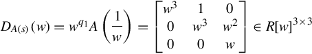
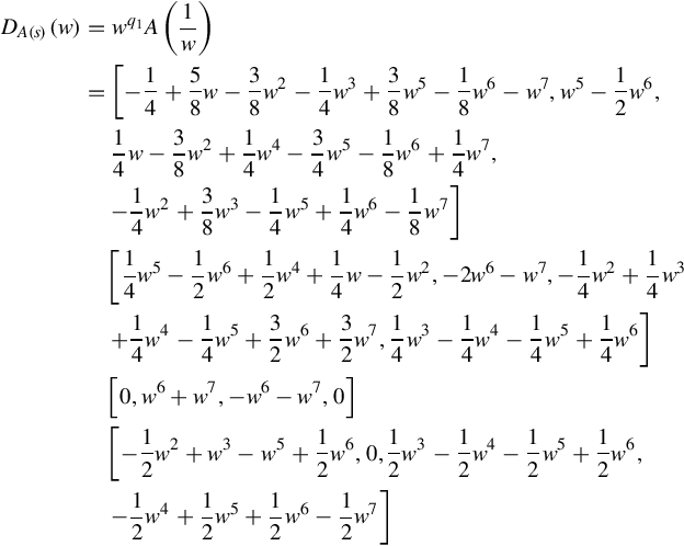
are the orders of the infinite zeros at ![]() of A(s). The dual polynomial of A(s) is defined as
of A(s). The dual polynomial of A(s) is defined as

The local Smith form of DA(s)(w) at w = 0 is

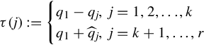
It is seen that the polynomial matrices have in general three kinds of IEDs, or equivalently DA(s)(w) has three kinds of finite zero at w = 0. The first kind of IEDs with orders q1 − qj, j = 2, 3, …, k correspond to the poles of A(s) at ![]() . The second kind of IEDs comprise those corresponding to the zeros of A(s) at
. The second kind of IEDs comprise those corresponding to the zeros of A(s) at ![]() with orders
with orders ![]() , j = r − h + 1, …, r. The third kind with orders q1 is not dynamically important [18].
, j = r − h + 1, …, r. The third kind with orders q1 is not dynamically important [18].
Let ![]() ,
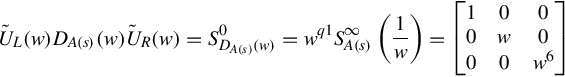
, ![]() be unimodular matrices reducing DA(s)(w) to its local Smith form
be unimodular matrices reducing DA(s)(w) to its local Smith form ![]() , i.e.,
, i.e.,
Let uj(w) ∈ R[w]r×1, vj(w) ∈ R[w]r×1, ![]() be the columns of
be the columns of ![]() and
and ![]() , then
, then
where
Let

then for j = 2, 3, …, r, the vectors
form a Jordan chain corresponding to the zero w = 0 of the IEDs wτ(j). Now we can compare the two different definitions of the infinite Jordan pair.
Definition 9.2.1
(Gohberg et al. [17])
The generalized infinite Jordan pair ![]() of A(s) are defined as
of A(s) are defined as
where

1. ![]() is nilpotent with an index of nil-potency
is nilpotent with an index of nil-potency ![]() , because the largest Jordan block is
, because the largest Jordan block is ![]() .
.
2. ![]() (the total number of the infinite poles of A(s))
(the total number of the infinite poles of A(s))![]() (the total number of the infinite zeros of A(s)).
(the total number of the infinite zeros of A(s)).

1. ![]() is nilpotent with an index of nil-potency
is nilpotent with an index of nil-potency ![]() , because the largest Jordan block is
, because the largest Jordan block is ![]() .
.
2. ![]() .
.
The above two interpretations of infinite Jordan pairs display an essential difference. For example, the roles that the infinite poles and the infinite zeros play in the system behaviors are considered in totally different manners. It is obvious that v ≥ μ, and the dimensions of the generalized infinite Jordan pair of Definition 9.2.1 are unnecessarily larger than that of the infinite Jordan pair of Definition 9.2.2 due to some redundant information being included. This can be seen clearly from the following example.
Example 9.2.1
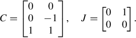
Consider the polynomial matrix
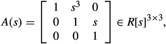
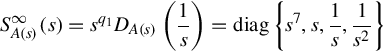
its Smith-McMillan form is

Thus A(s) has two infinite poles at degrees 1 and 3 and an infinite zero at degree 4. The dual polynomial matrix to A(s) is
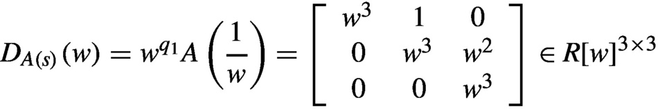
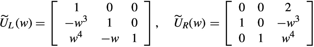
and
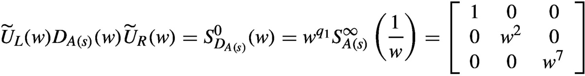
is the local Smith form of DA(S)(w) at w = 0, where
So we get three kinds of infinite elementary divisor:
• w2 corresponding to the infinite pole of A(s),
• w7 corresponding to the infinite zero of A(s) and the IED 1 = w0.
From

we have

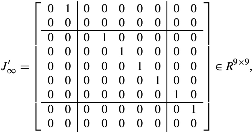
According to Definition 9.2.1, the generalized infinite Jordan pair in the sense of Gohberg et al. [17] is ![]() :
:

While the infinite Jordan pair in the sense of Vardulakis [13] is ![]() with:
with:

In the above example it is noted that the dimensions of the generalized infinite Jordan pair, which are 3 × 9 and 9 × 9, are unnecessarily larger than that of the infinite Jordan pair, which are 3 × 5 and 5 × 5. Such a tendency will become more evident as the number of the infinite poles of A(s), the dimension of A(s) and the degree of A(s) are increased. However, the following observation arising from the above two definitions of infinite Jordan pairs suggests the possibility of deleting the redundant information that is contained in the generalized infinite Jordan pair.
Theorem 9.2.1
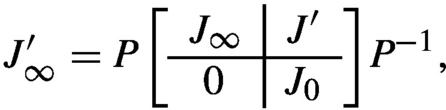
If ![]() is a generalized infinite Jordan pair, there exists an elementary matrix P such that
is a generalized infinite Jordan pair, there exists an elementary matrix P such that
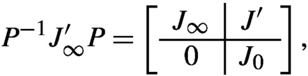
where C0 ∈ Rr×(v−μ), J′∈ Rμ×(v−μ), J0 ∈ R(v−μ)×(v−μ), 0 ∈ R(v−μ)×μ and ![]() is an infinite Jordan pair. Furthermore, J0 is nilpotent with an index of nil-potency q1 − 1.
is an infinite Jordan pair. Furthermore, J0 is nilpotent with an index of nil-potency q1 − 1.
Proof
Note that ![]() is a submatrix of
is a submatrix of ![]() . By a series of interchanging of two columns in
. By a series of interchanging of two columns in ![]() ,
, ![]() can be brought to the form
can be brought to the form ![]() . We denote this elementary matrix as P, then
. We denote this elementary matrix as P, then ![]() , where C0 ∈ Rr×(v−μ). Similarly, by interchanging the corresponding columns and the corresponding rows of
, where C0 ∈ Rr×(v−μ). Similarly, by interchanging the corresponding columns and the corresponding rows of ![]() can be brought to a block matrix, i.e.,
can be brought to a block matrix, i.e.,

where

It can easily be seen that J0 is nilpotent with an index of nil-potency q1 − 1.
Remark 9.2.1
The above elementary matrix P has the effect of deleting the redundant information in two ways. First, it deletes the redundant information in those blocks in the infinite Jordan pair of Gohberg et al. [17] that corresponds to the infinite zeros and brings them to the correct sizes. Second, it deletes all blocks in ![]() that correspond to the infinite poles and all blocks that are not dynamically important. In this way the resulting resolvent decomposition more precisely reflects the relevant system structure, since the deleted blocks in the infinite Jordan pairs display no dynamics in the state solution. This will be seen explicitly when the effect of P on Z has been determined in a subsequent result.
that correspond to the infinite poles and all blocks that are not dynamically important. In this way the resulting resolvent decomposition more precisely reflects the relevant system structure, since the deleted blocks in the infinite Jordan pairs display no dynamics in the state solution. This will be seen explicitly when the effect of P on Z has been determined in a subsequent result.
Example 9.2.2
Recall Example 9.2.1, we have
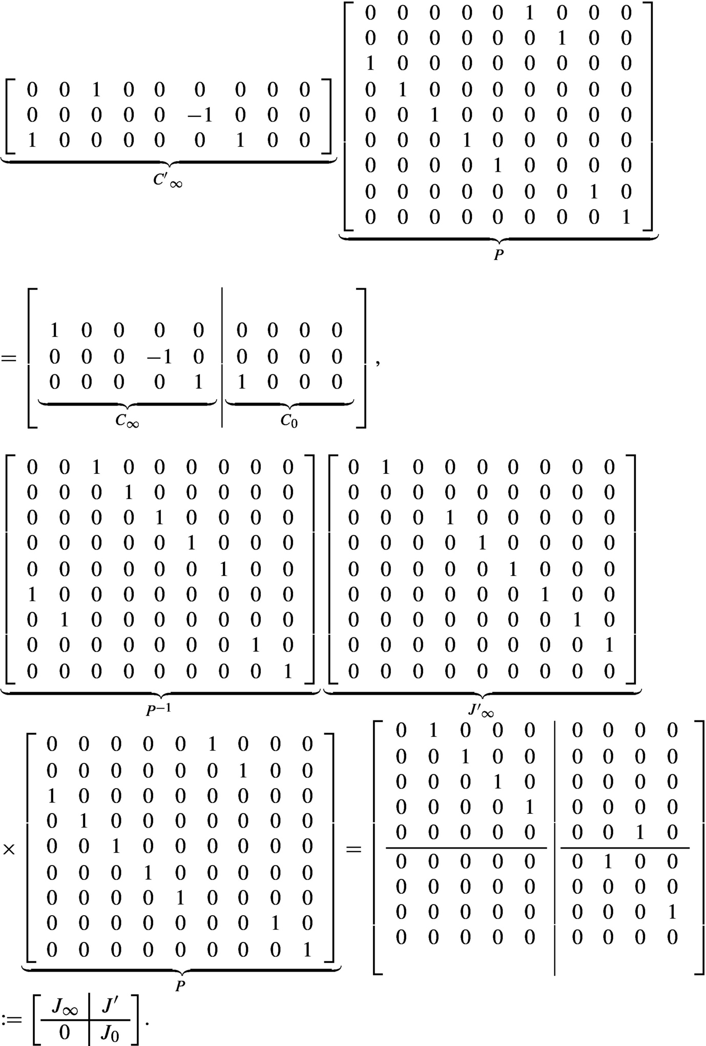
It is noted that here J0 is nilpotent with index of nil-potency 2.
The key point in here is to find the above elementary matrix P to delete the redundant information. Based on the information carried by the Smith-McMillan form at ![]() of A(s), P results from a series of elementary operations from an identity matrix, which is very easy to obtain. Once the redundant information is deleted from the generalized infinite Jordan pair, the generalized infinite Jordan pair and the elementary matrix P are not involved in computation in the solution procedure.
of A(s), P results from a series of elementary operations from an identity matrix, which is very easy to obtain. Once the redundant information is deleted from the generalized infinite Jordan pair, the generalized infinite Jordan pair and the elementary matrix P are not involved in computation in the solution procedure.
9.3 The solution of regular PMDs
We consider now the homogeneous regular PMD:
Let ![]() be the Smith-McMillan form at
be the Smith-McMillan form at ![]() of
of ![]() :
:

and if A(s) has at least one zero at ![]() then the Laurent expansion of A−1(s) can be written as follows
then the Laurent expansion of A−1(s) can be written as follows

where ![]() is the polynomial part of A−1(s) and Hsp(s) ∈ Rr×r(s) is the strictly proper part of A−1(s). Let a resolvent decomposition of A(s) be given by
is the polynomial part of A−1(s) and Hsp(s) ∈ Rr×r(s) is the strictly proper part of A−1(s). Let a resolvent decomposition of A(s) be given by
where ![]() . It should be noted that (C, J, Z1) is a realization of Hsp(s), and
. It should be noted that (C, J, Z1) is a realization of Hsp(s), and ![]() is a realization of Hpol(s). Considering the Laplace transformation of Eq. (9.4), we obtain
is a realization of Hpol(s). Considering the Laplace transformation of Eq. (9.4), we obtain
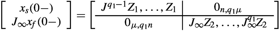
where ![]() is the initial condition vector associated with the initial values of ξ(t) and its (q1 − 1)-derivatives at t = 0 −, i.e.,
is the initial condition vector associated with the initial values of ξ(t) and its (q1 − 1)-derivatives at t = 0 −, i.e., ![]() given by Fossard [108], Pugh [107]
given by Fossard [108], Pugh [107]
 (9.6)
(9.6)
We obtain
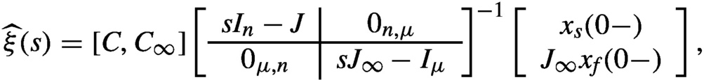 (9.7)
(9.7)
where the vector
 (9.8)
(9.8)
Now by taking the inverse L− Laplace transformation of Eq. (9.7), we have the following result.
Lemma 9.3.1
(Vardulakis [13])
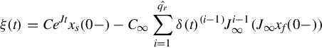
The general solution of homogeneous PMD (Eq. 9.4) is

where δ(t) is the Dirac impulse function.
The next result constructs a resolvent decomposition for a regular polynomial matrix, which follows from Gohberg et al. [17].
Lemma 9.3.2
Let ![]() ,
, ![]() . If (C, J) is the finite Jordan pair of A(s), and
. If (C, J) is the finite Jordan pair of A(s), and ![]() is the generalized infinite Jordan pair of A(s) in the sense of Gohberg et al. [17],
is the generalized infinite Jordan pair of A(s) in the sense of Gohberg et al. [17], ![]() . Put
. Put
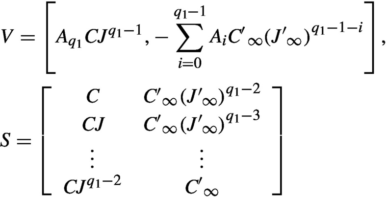
and
 (9.9)
(9.9)
then
 (9.10)
An interesting observation from Eq. (9.9) is the following.

Proof
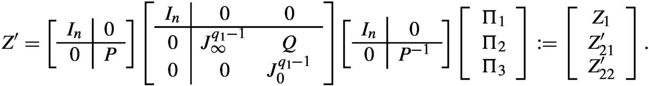
Let
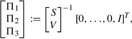
where Π1 ∈ Rn×1, Π2 ∈ Rμ×1, Π3 ∈ R(v−μ)×1. From Theorem 9.2.1, there exists an elementary matrix P ∈ Rv×v, such that
so

where ![]() .
.
Noticing J0 is nilpotent with an index of nil-potency q1 − 1, i.e., ![]() it follows that:
it follows that:

The above observation is interesting, not least for the way in which the redundant information contained in ![]() is deleted. More importantly than this, however, is that such a mechanism of decoupling makes the computation of P attractive and facilitates the proposed refined resolvent decomposition.
is deleted. More importantly than this, however, is that such a mechanism of decoupling makes the computation of P attractive and facilitates the proposed refined resolvent decomposition.
The following result proposes a new approach to constructing a resolvent decomposition in terms of the finite Jordan pair, the infinite Jordan pair and the generalized infinite Jordan pair, which is fundamental for us to formulate the solution of the PMD. As one of our main results, we are ready to state it as follows.
Theorem 9.3.1
If (C, J) is the finite Jordan pair of A(s) and (![]() ) is the infinite Jordan pair of A(s) in the sense of Vardulakis [13],
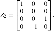
) is the infinite Jordan pair of A(s) in the sense of Vardulakis [13], 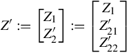 is given by Lemma 9.3.2, let Z2 ∈ Rμ×r be given by
then
 (9.11)

Remark 9.3.1
The resolvent decomposition proposed by Vardulakis [13] reflects the system solution structure precisely; however, the realization approach is not so straightforward by itself. On the other hand in the resolvent decomposition proposed by Gohberg et al. [17] (Lemma 9.3.2), ![]() were formulated explicitly. However, there is some redundant information as described in Theorem 9.2.1 and it does not give such a precise insight into the system structure. The resolvent decomposition proposed here is a refinement of these two results and inherits the advantages of both results. Due to the fact that the redundant information is deleted, the proposed refined resolvent decomposition has minimal dimensions, the proposed approach has an obvious advantage, i.e., computation of the inverse matrix of A(s) can be carried out more efficiently.
were formulated explicitly. However, there is some redundant information as described in Theorem 9.2.1 and it does not give such a precise insight into the system structure. The resolvent decomposition proposed here is a refinement of these two results and inherits the advantages of both results. Due to the fact that the redundant information is deleted, the proposed refined resolvent decomposition has minimal dimensions, the proposed approach has an obvious advantage, i.e., computation of the inverse matrix of A(s) can be carried out more efficiently.
For the nonhomogeneous regular PMD
the following theorem gives the complete solution.
Theorem 9.3.2
Let ![]() be regular, and let
be regular, and let ![]() be the Smith-McMillan form of A(s) at
be the Smith-McMillan form of A(s) at ![]() . If (C, J) is the finite Jordan pair of A(s) and (
. If (C, J) is the finite Jordan pair of A(s) and (![]() ) is the infinite Jordan pair of A(s) (in the sense of Vardulakis [13]), (C, J, Z1) and (
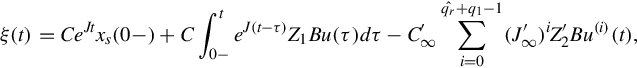
) is the infinite Jordan pair of A(s) (in the sense of Vardulakis [13]), (C, J, Z1) and (![]() ) satisfy the resolvent decomposition (Eq. 9.11), then the complete solution of regular PMD (Eq. 9.12) is
) satisfy the resolvent decomposition (Eq. 9.11), then the complete solution of regular PMD (Eq. 9.12) is

where ![]() are initial values given by Eq. (9.8).
are initial values given by Eq. (9.8).
Proof
From Lemma 9.3.1, one knows that
generates the general solution of the homogeneous PMD, so we only need to check that the formula (9.13) does indeed produce a solution of the nonhomogeneous PMD (Eq. 9.12). To this end, when t > 0, we have
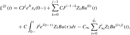
so

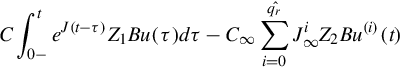
Using the property ![]() and rearranging the terms, we have
and rearranging the terms, we have

Noticing

from
it follows that

Hence
which finishes the proof.
Remark 9.3.3
The above solution displays precisely the zero state response by means of
and the zero input response through the term

Also the impulsive properties of the system are displayed in this solution due to the fact that the initial conditions of the pseudo-state are considered. Such an impulsive part to the general nonhomogeneous PMDs solution is, however, unavailable from the solution of Gohberg et al. [17] and Vardulakis [13].
Remark 9.3.4
According to Gohberg et al. [17], the solution of PMD (Eq. 9.12) is following (without the impulse solution part):
where (![]() ) is the infinite Jordan pair in the sense of Gohberg et al. [17].
) is the infinite Jordan pair in the sense of Gohberg et al. [17]. ![]() are given by Eq. (9.9). By using Theorem 9.2.1, Proposition 9.3.1 and noticing that
are given by Eq. (9.9). By using Theorem 9.2.1, Proposition 9.3.1 and noticing that ![]() is nilpotent with an index of nil-potency
is nilpotent with an index of nil-potency ![]() , one finds that
, one finds that
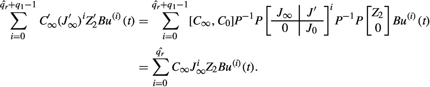
It is thus clearly seen that the redundant information included in the solution of Gohberg et al. [17] due to using the generalized infinite Jordan pairs does not appear in our solution any more. Also this helps to clarify the mechanism of decoupling in the solution of Gohberg et al. [17].
By comparing our solution with the solution of Gohberg et al. [17] and the solution of Vardulakis [13], it can be seen that, besides the fact that it displays the impulsive solution part, our solution can be carried out more efficiently in actual computation. The main reason for this is that the refined resolvent decomposition does not contain any redundant information, since the infinite Jordan pairs used in our solution are of minimal dimensions, and the matrices Z1 and Z2 are formulated explicitly. The refined resolvent decomposition facilitates computation of the inverse matrix of A(s) because the dimension of the matrices used are minimal. Rather than calculating the inverse matrix A−1(s) with an overly large dimension, it is suggested first to calculate the easily available elementary matrix P to delete all redundant information and then to obtain the inverse matrix with the minimal dimension. Once the refined resolvent decomposition is obtained, the generalized infinite Jordan pair and the elementary matrix P are not necessary for the calculation of the solution of the regular PMD. This thus presents another advantage of this method, which is algorithmically attractive when applied in actual computation.
9.4 Algorithm and examples
As mentioned before, the refined resolvent decomposition plays a key role in our approach, the difficulty in obtaining the solution of the regular PMDs depends on the calculation of this refined resolvent decomposition. To help clarify the construction of this refined resolvent decomposition, for the implementation of Theorem 9.3.1, the following algorithm is now given, which is useful for symbolic computational packages Maple.
Algorithm 9.4.1
(Computation of the refined resolvent decomposition of A(s) ∈ R[s]r×r)
Step 1 Let A(s) = ∑i=0q1Aisi, calculate the Smith form and the finite Jordan pair (C, J).
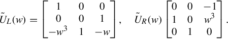
Step 2 Find the dual polynomial DA(s)(w) of A(s), calculate the local Smith form of DA(s)(w) at w = 0 SDA(s)0(w) and the unimodular matrices ŨL(w), ŨR(w) such that
Step 3 Differentiate the matrix ŨR(w) and then construct the generalized infinite Jordan pair (C∞′, J∞′) and the infinite Jordan pair (C∞, J∞).
Step 4 Find the elementary matrix P by using Theorem 9.2.1.
Step 5 Calculate V, S and Z′ by Lemma 9.3.2.
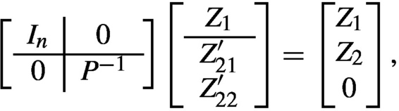
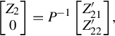
Step 6 Partition Z′ = [Z1Z2′] = [Z1Z21′Z22′], from [Z20] = P−1 [Z21′Z22′] calculate Z2.
Step 7 Finally, obtain the refined resolvent decomposition
Example 9.4.1
Let

with

r = 3, n = deg det(A(s)) = 2. The finite Jordan pairs of A(s) is (C, J):
The Smith-McMillan form of A(s) at ![]() is
is
so A(s) has two poles at ![]() with orders q1 = 3 and q2 = 2 respectively and one zero at
with orders q1 = 3 and q2 = 2 respectively and one zero at ![]() with orders
with orders ![]() . The dual polynomial matrix to A(s) is
. The dual polynomial matrix to A(s) is
and
is the local Smith form of DAs(w) at w = 0, where
One easily obtains the generalized infinite Jordan pair (![]() ) (in the sense of Gohberg et al. [17]) of A(s) as following
) (in the sense of Gohberg et al. [17]) of A(s) as following
 (9.14)
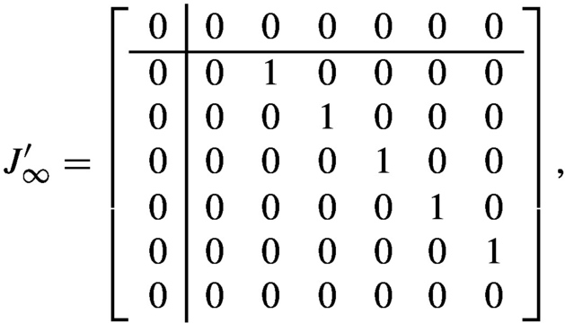 (9.15)
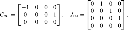
and the infinite Jordan pair(![]() ) (in the sense of Vardulakis [13]) of A(s) as
) (in the sense of Vardulakis [13]) of A(s) as
It is easy to find P,

such that
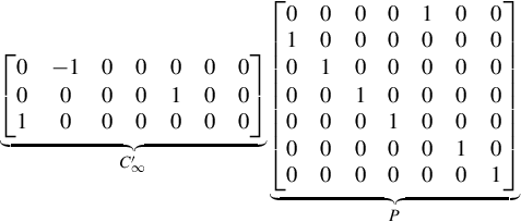
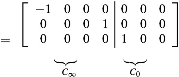
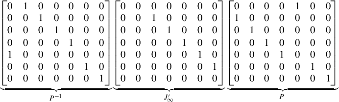

According to Lemma 9.3.2, one has

so
 (9.16)
We obtain
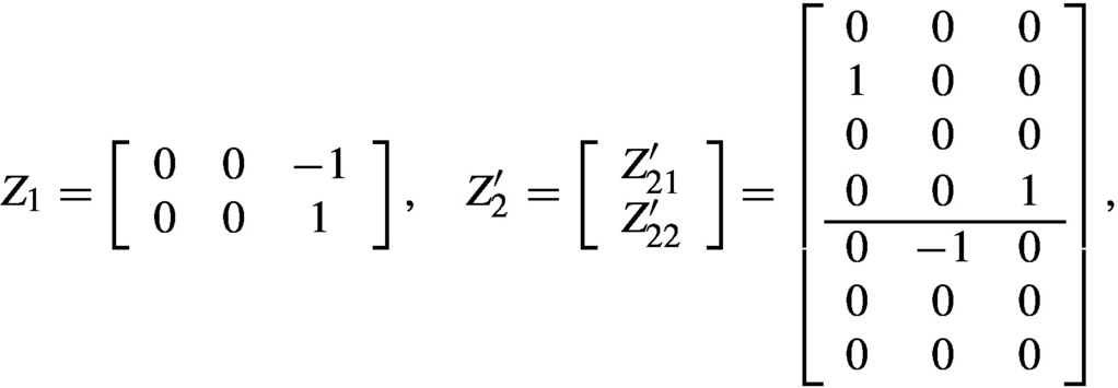
and from
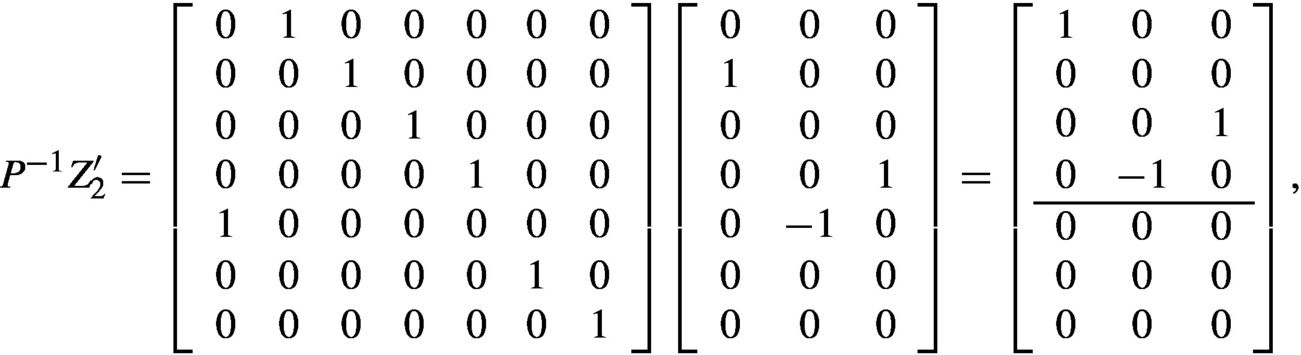
we obtain
Hence, by Theorem 9.3.1 we have constructed a resolvent form for the regular polynomial matrix A(s) as following

Note that in the above refined resolvent decomposition the matrices ![]() and Z2 have the minimal dimensions of 3 × 4, 4 × 4, and 4 × 3. Compared to the resolvent decomposition of Gehberg et al. [17] given by
and Z2 have the minimal dimensions of 3 × 4, 4 × 4, and 4 × 3. Compared to the resolvent decomposition of Gehberg et al. [17] given by
where ![]() ,
, ![]() , and
, and ![]() are given by Eqs. (9.14), (9.15), (9.16), respectively, due to the fact that the redundant information has been deleted, the above refined resolvent decomposition is obviously in a much more concise form which will definitely bring some convenience when applied to the solution of the regular PMDs.
are given by Eqs. (9.14), (9.15), (9.16), respectively, due to the fact that the redundant information has been deleted, the above refined resolvent decomposition is obviously in a much more concise form which will definitely bring some convenience when applied to the solution of the regular PMDs.
Example 9.4.2
Consider the following regular polynomial matrix
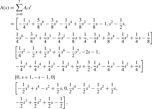
r = 4, q1 = 7, n = deg det(A(s)) = 5. The finite Jordan pairs of A(s) is (C, J):
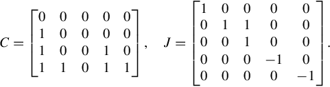
The dual polynomial matrix to A(s) is
and

is the local Smith form of DA(s)(w) at w = 0. The Smith-McMillan form of A(s) at ![]() is
is
so A(s) has two poles at ![]() with orders q1 = 7 and q2 = 1 respectively and two zeros at
with orders q1 = 7 and q2 = 1 respectively and two zeros at ![]() with orders
with orders ![]() and
and ![]() respectively
respectively

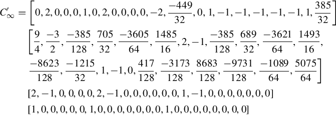
Use the local Smith form of DA(s) at w = 0 to find the generalized infinite Jordan pair (![]() ) (in the sense of Gohberg et al. [17]) of A(s):
) (in the sense of Gohberg et al. [17]) of A(s):