
Fundamental approaches to control system analysis
Keywords
Control system analysis; Polynomial matrix description; Linear multivariable control systems; Behavioral approach; Chain-scattering representations
The main purpose of this introductory chapter is to familiarize the reader with such basic theories on control system structure and behavior as the polynomial matrix description (PMD) theory, behavioral theory, and chain-scattering representation (CSR) approaches. This chapter also serves to prepare for the representation of our results in the succeeding chapters.
6.1 PMD theory of linear multivariable control systems
The main aim of this section is to briefly introduce the background and preliminary results in PMD theory, which are needed in the sequel of this book. Regarding the related issue of determination of finite and infinite frequency structure of a rational matrix and the issue of the resolvent decomposition and solution of regular PMD, this book will present its contributions in Chapters 7–10. The main references to the following introduction are Rosenbrock [5], Vardulakis [13], and Kailath [32].
The initial aim [5] of PMD theory was to describe various time domain results of Kalman’s state space theory into a powerful algebraic language by using the existing results in matrix theory. This led to a better understanding of the mathematical structure of linear multivariable systems by generalizing the classical single-input single-output transfer function approaches to multivariable case. It finally resulted in various synthesis techniques for multivariable feedback systems. So far PMD theory has been established as a very successful and still developing area in the linear multivariable control system theory.
Throughout this book, ![]() denotes the set of p × q polynomial matrices, while
denotes the set of p × q polynomial matrices, while ![]() denotes the set of p × q rational matrices. Regular (PMDs) or linear nonhomogeneous matrix differential equations (LNHMDEs) are described by
denotes the set of p × q rational matrices. Regular (PMDs) or linear nonhomogeneous matrix differential equations (LNHMDEs) are described by
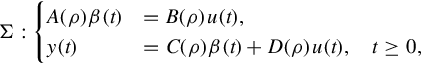
where ρ := d/ dt is the differential operator, ![]() ,
, ![]() ,
, ![]() ,
, ![]() ,
, ![]() is the pseudo-state of the PMDs,
is the pseudo-state of the PMDs, ![]() is a p times piecewise continuously differentiable function called the input,
is a p times piecewise continuously differentiable function called the input, ![]() is the output vector of the PMD.
is the output vector of the PMD.
Taking the Laplace transform of Eq. (6.1) and assuming “zero initial conditions,” i.e., that
Eq. (6.1) can be written as

where ![]() ,
, ![]() ,
, ![]() are Laplace transforms of β(t), u(t), and y(t), respectively. From Eq. (6.2) we have
are Laplace transforms of β(t), u(t), and y(t), respectively. From Eq. (6.2) we have
A polynomial matrix ![]() is called
is called ![]() -unimodular or simply unimodular if there exists a matrix
-unimodular or simply unimodular if there exists a matrix ![]() such that
such that ![]() , where Ip denotes the p × p identity matrix, equivalently if
, where Ip denotes the p × p identity matrix, equivalently if ![]() .
.
Definition 6.1.2
The degree of a polynomial matrix ![]() , denoted by deg T(s), is defined as the maximum degree among the degrees of all its maximum order (nonzero) minors.
, denoted by deg T(s), is defined as the maximum degree among the degrees of all its maximum order (nonzero) minors.
Corollary 6.1.1
If T(s) is a nonsingular square polynomial matrix, then
where ![]() denotes the determinant of the indicated matrix.
denotes the determinant of the indicated matrix.
Corollary 6.1.2
![]() is unimodular if and only if deg T(s) = 0.
is unimodular if and only if deg T(s) = 0.
Two rational matrices T1(s), ![]() are called equivalent if there exist unimodular matrices
are called equivalent if there exist unimodular matrices ![]() such that
such that
Any rational matrix is equivalent to its Smith-McMillan form, which is a canonical form of a matrix.
Theorem 6.1.1
([5] Smith-McMillan form of a rational matrix in C)
Let ![]() with
with ![]() ,
, ![]() . Then T(s) is equivalent to a diagonal matrix
. Then T(s) is equivalent to a diagonal matrix ![]() having the form
having the form
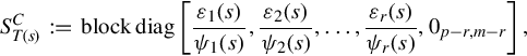
where ![]() are monic and coprime such that εi(s) divides εi+1(s), and Ψi+1(s) divides Ψi(s), i = 1, 2, …, r − 1.
are monic and coprime such that εi(s) divides εi+1(s), and Ψi+1(s) divides Ψi(s), i = 1, 2, …, r − 1.
If ![]() then Ψi(s) = 1, ∀i ∈r, that is,
then Ψi(s) = 1, ∀i ∈r, that is, ![]() is also a polynomial matrix and it is called the Smith form of T(s). Otherwise, i.e., if T(s) is nonpolynomial, for some i and j, Ψi(s) are nonconstant, that is
is also a polynomial matrix and it is called the Smith form of T(s). Otherwise, i.e., if T(s) is nonpolynomial, for some i and j, Ψi(s) are nonconstant, that is ![]() is also nonpolynomial and it is called McMillan form of T(s).
is also nonpolynomial and it is called McMillan form of T(s).
The zeroes of T(s) are defined as the zeros of the polynomials εi(s), i ∈r. The poles of T(s) are defined as the zeros of the polynomials Ψi(s), i ∈r.
Vardulakis et al. [87] introduced the concept of the Smith-McMillan form at infinity of a rational matrix. The main definitions are briefly presented here.
Definition 6.1.3
![]() will be called proper if
will be called proper if ![]() exists. If the limit is zero then T(s) will be called strictly proper , while if this limit is nonzero T(s) will be called exactly proper .
exists. If the limit is zero then T(s) will be called strictly proper , while if this limit is nonzero T(s) will be called exactly proper .
Let ![]() denote the ring of proper rational functions.
denote the ring of proper rational functions.
Definition 6.1.4
The m × m rational matrix ![]() is said to be biproper if and only if
is said to be biproper if and only if
2. ![]() .
.
The p ×m rational matrices T1(s) and T2(s) are said to be equivalent at infinity if there exist biproper matrices ![]() such that
such that
Since W(s) and V (s) are biproper, it can be seen from Definition 6.1.4 that W(s) and V (s) possess neither poles nor zeros at infinity. It therefore follows intuitively from this that T1(s) and T2(s) have an identical pole-zero structure at infinity. A canonical form for a rational matrix under the equivalence at infinity is its Smith-McMillan form at infinity, ![]() .
.
Theorem 6.1.2
(Smith-McMillan form of a rational matrix at ![]() )
)
Let ![]() with
with ![]() . Then T(s) is equivalent at
. Then T(s) is equivalent at ![]() to a diagonal matrix having the form
to a diagonal matrix having the form
where 1 ≤ k ≤ r and
are respectively the orders of its poles and zeros at ![]()
A reduction approach for computing Smith-McMillan form at ![]() of a rational matrix is suggested in [87].
of a rational matrix is suggested in [87].
Any rational function can be represented as a ratio of coprime polynomials, this can be generalized to the matrix case.
Definition 6.1.5
Let ![]() with
with ![]() ,
, ![]() Then there exist nonunique pairs:
Then there exist nonunique pairs: ![]() ,
, ![]() and left coprime,
and left coprime, ![]() ,
, ![]() and right coprime such that
and right coprime such that
A representation of a rational matrix T(s) given by Eq. (6.6) is called a left (right) coprime polynomial matrix fraction description (MFD) of T(s).
Let A(s) ∈ R[s]r×r, ![]() . Then by Theorem 6.1.2A(s) is equivalent at
. Then by Theorem 6.1.2A(s) is equivalent at ![]() to its Smith-McMillan form
to its Smith-McMillan form ![]() having the form
having the form
where 1 ≤ k ≤ r and
If A(s) has at least one zero at ![]() , let
, let
be the Laurent expansion of A(s)−1 at ![]() , where k > 0, Hk≠0. Then one has
, where k > 0, Hk≠0. Then one has
Let
![]() and λ0 ∈ C such that
and λ0 ∈ C such that ![]() . The sequence of r-dimensional vectors x0, x1, …, xm(x0≠0) for which the following equalities hold
. The sequence of r-dimensional vectors x0, x1, …, xm(x0≠0) for which the following equalities hold
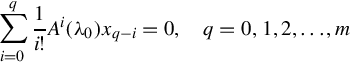
is called a Jordan Chain of length (m + 1) for A(s) corresponding to λ0. Now let
1 ≤ k ≤ r be the Smith Form of A(s).
Let
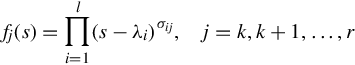
be the decomposition of the invariant polynomials fj(s) into irreducible elementary divisors over C, i.e., assure that
has l distinct zeroes
where
are the partial multiplicities of the eigenvalues λi. Let
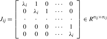
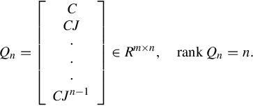
be the Jordan Chain of lengths σij corresponding to the eigenvalue λi of A(s) and consider the matrices
where ![]() and
and
where
Definition 6.1.7
Let T(s) ∈ Rpr(s)p×m, then a quadruple (A, B, C, E) such that
is called a realization of the proper rational matrix T(s).
Definition 6.1.8
A realization (A, B, C, E) of a T(s) ∈ Rpr(s)p×m is called a minimal realization of T(s) if
where δM(T(s)) is the McMillan degree of T(s).
Definition 6.1.9
Let T(s) ∈ R[s]p×m. Then a triple of matrices ![]() ,
, ![]() ,
, ![]() such that
such that
is called a realization of the polynomial matrix T(s).
A realization of T(s) ∈ R[s]p×m can always be obtained from a realization of the strictly proper rational matrix ![]() . Because if
. Because if ![]() , is a realization of
, is a realization of ![]() , i.e., if
, i.e., if
then Eq. (6.12) by the substitution ![]() gives Eq. (6.11).
gives Eq. (6.11).
Proposition 6.1.2
(Vardulakis [13])
Let
its Smith-McMillan form at infinity is
are respectively the orders of its poles and zeros at ![]() . Then
. Then
1. The McMillan degree of ![]() is given by
is given by
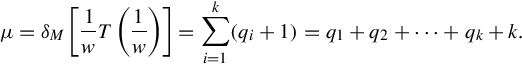
2. If ![]() is a minimal realization of T(s) with
is a minimal realization of T(s) with ![]() in Jordan form, then
in Jordan form, then
where

Crucial to the issue of the solution of regular PMDs, which we will discuss later, is the concept of an infinite Jordan pair of a regular polynomial matrix, i.e., a Jordan pair ![]() ,
, ![]() which corresponds to its zeros at
which corresponds to its zeros at ![]() .
.
Definition 6.1.10
([17])
Let ![]() ,
, ![]() Then a pair
Then a pair

![]() is called an infinite Jordan pair of A(s) if it is a (finite) Jordan pair of the “dual” polynomial matrix
is called an infinite Jordan pair of A(s) if it is a (finite) Jordan pair of the “dual” polynomial matrix
corresponding to its zero at w = 0, or equivalently if and only if (by Proposition 6.1.1)
and

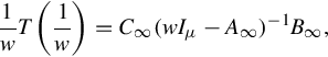
Regarding the resolvent decomposition of a regular polynomial matrix which is closely related to the solution of regular PMD, Vardulakis [13] gave the following result.
Theorem 6.1.3
Let ![]() with Smith-McMillan form at
with Smith-McMillan form at ![]() given by Eq. (6.7). Write
given by Eq. (6.7). Write
where ![]() and
and ![]() is strictly proper.
is strictly proper.
Let ![]()
![]() Let
Let ![]() be a minimal realization of Hsp(s) and
be a minimal realization of Hsp(s) and ![]() be a minimal realization of Hpol(s). Then C, J is a finite Jordan pair of A(s) and
be a minimal realization of Hpol(s). Then C, J is a finite Jordan pair of A(s) and ![]() is an infinite Jordan pair of A(s). Furthermore, A(s)−1 can be written as
is an infinite Jordan pair of A(s). Furthermore, A(s)−1 can be written as
 (6.13)
6.2 Behavioral approach in systems theory
The purpose of this section is to briefly introduce behavioral theory. Based on these preliminary results we will present a new approach realization of behavior in Chapter 12. The main references to the following introduction are [26, 27, 88, 89].
Both the transfer function and the state space approaches view a system as a signal processor that accepts inputs and transfers them into outputs. In the transfer function approach, this processor is described through the way in which exponential inputs are transformed into exponential outputs. In the state space approach, this processor involves the state as an intermediate variable, but the ultimate aim remains to describe how inputs lead to outputs. This input-output point of view has played an important role in system control theory. However, the starting point of behavioral theory is fundamentally different. As claimed in [27, 28], such a starting point is more suited to modeling and more suitable for actual applications in certain circumstances.
In the behavioral approach a mathematical model is viewed as a subset of a universum of possibilities. Before one accepts a mathematical model as a description of reality, all outcomes in the universum are in principle possible. After one accepts the mathematical model as a convenient description, one can declare that only outcomes in a certain subset are possible. This subset is called the behavior of the mathematical model. Starting from this perspective, one arrives at the notion of a dynamical system as simply a subset of time-trajectories, as a family of time signals taking on values in a suitable signal space.
It is in terms of the time trajectories of a specific system that all the concepts in behavioral theory are put forward. Linear time-invariant differential systems have such a nice structure that they fall into the scope of behavioral approach immediately. When one has a set of variables that can be described by such a system, then there is a transparent way of describing how trajectories in the behavior are generated. Some of the variables, it turns out, are free, i.e., unconstrained. They can thus be viewed as unexplained by the model and imposed on the system by the environment. These variables are called inputs. Once these variables are determined, the remaining variables called outputs are not yet completely specified, because of the possible trajectories, which are dependent on the past history of the system. This means that the outputs are still dependent on the initial conditions of the system. To formulate this relationship between the outputs, the inputs and the initial conditions of the system, one thus has to use the concept of state.
When one models an interconnected physical system, then unavoidably auxiliary variables, in addition to the variables modeled, will appear in the model. In order to distinguish them from themanifest variables, which are the variables whose behavior the model aims to describe, these auxiliary variables are called latent variables. The interaction between manifest and latent variables is one of the themes in this book. In this book a new approach, realization of behavior, will be presented to expose this interaction. In [27] it was shown how to eliminate latent variables and how to introduce state variables. Thus a system of linear differential equations containing latent variables can be transformed in an equivalent system in which these latent variables have been eliminated.
The basic idea in our approach of realization of behavior is, however, to find an ARMA representation for a given frequency behavior description such that the known frequency behavior is completely recovered to the corresponding dynamical behavior. From this point of view, realization of behavior is seen to be a converse procedure to the above latent variable eliminating process. Such a realization approach is believed to be highly significant in modeling dynamical system in some real cases where the system behavior is conveniently described in the frequency domain. Since no numerical computation is required of the procedure, the realization of behavior is believed to be particularly suitable for situations in which the coefficients are symbolic rather than numerical.
Definition 6.2.1
([89])
Let ![]() be a universum,
be a universum, ![]() a set, and
a set, and ![]() . The mathematical model
. The mathematical model ![]() with
with ![]() is said to be described by behavioral equations and is denoted by
is said to be described by behavioral equations and is denoted by ![]() . The set
. The set ![]() is called the equating space. We also call
is called the equating space. We also call ![]() a behavioral equation representation of
a behavioral equation representation of ![]() .
.
Latent variables appear frequently in system modeling practice, for which examples abound and are provided in [27, 89]. The need to use latent variables is recognized from the situations where for mathematical reasons they are unavoidably involved in expressing the basic laws in the modeling process. For example, state variables are needed in system theory in order to express the memory of a dynamical system, internal voltages and currents are needed in electrical circuits in order to express the external port behavior, momentum is needed in Hamiltonian mechanics in order to describe the evolution of the position, prices are needed in economics in order to explain the production and exchange of economic goods, etc.
Definition 6.2.2
([89])
A mathematical model with latent variables is defined as a triple ![]() with
with ![]() the universum of manifest variables,
the universum of manifest variables, ![]() the universum of latent variables, and
the universum of latent variables, and ![]() the full behavior. It defines the manifest mathematical model
the full behavior. It defines the manifest mathematical model ![]() with
with ![]() such that
such that ![]() ;
; ![]() is called the manifest behavior (or the external behavior) or simply the behavior. We call
is called the manifest behavior (or the external behavior) or simply the behavior. We call ![]() a latent variable representation of
a latent variable representation of ![]() .
.
Now by applying the above ideas the following basic description about dynamical system can be set up in a language of behavioral theory.
Definition 6.2.3
([27])
A dynamical system Σ is defined as a triple
with ![]() a subset of
a subset of ![]() , called the time axis,
, called the time axis, ![]() a set called the signal space, and
a set called the signal space, and ![]() is a subset of
is a subset of ![]() called the behavior.
called the behavior.
Now consider the following class of dynamical systems with latent variables
where ![]() is the trajectory of the manifest variables, whereas
is the trajectory of the manifest variables, whereas ![]() is the trajectory of the latent variables. The equating space is
is the trajectory of the latent variables. The equating space is ![]() , and the behavioral equations are parameterized by the two polynomial matrices
, and the behavioral equations are parameterized by the two polynomial matrices ![]() and
and ![]() .
.
The question of elimination of latent variables is, what sort of behavioral equation does Eq. (6.14) imply about the manifest variable w alone? In particular, we wonder whether the relations imposed on the manifest variable w by the full behavioral equations (6.14) can themselves be written into the form of a system of differential equations. In other words, this question is to ask whether or not the set

can be written as the (weak) solution set of a system of linear differential equations. The above question is very important in situations where one has to introduce more variables in order to obtain a model of the relation between certain variables in a system of some complexity, after one proposes this model those auxiliary variables in which one is not interested may be eliminated by manipulating the equations (model).
An appealing and insightful answer to the above question is the following latent variable elimination procedure [27].


6.3 Chain-scattering representations
The main aim of this section is to briefly introduce some background and preliminary results on the CSR, which have been widely used in circuit theory, signal processing, and ![]() control theory. In Chapters 11 and 12 we will present some generalizations to these results. The main references to the following introduction are [21, 22, 90].
control theory. In Chapters 11 and 12 we will present some generalizations to these results. The main references to the following introduction are [21, 22, 90].
There are two basic interconnections widely used in circuit theory and signal processing. One is the series-parallel interconnection which is shown in Fig. 6.2, the other one is the cascade connection which is shown in Fig. 6.2.
Consider two well-defined n-ports in Fig. 6.1, both having the same numbers of series ports on the one hand, and of shunt ports on the other, and designate by H1 and H2 their hybrid matrices. It has been proved [21] that if the shunt ports are paralleled (port by port) and if the series ports are connected in series, the resulting n-port has the hybrid matrix

Generally one comes to the conclusion that impedance matrices (when they exist) add up for series connections at all ports, and admittance matrices add up for parallel connections.
In addition to the above series-parallel interconnection, it is often convenient to consider a cascade (or chain) connection of two subnetworks which is shown in Fig. 6.2, where the output ports of the first subnetwork are identical to the input ports of the second subnetwork. Let xa, xb, and xc be the electrical variables at the input ports of the first subnetwork, at the interconnected ports, and at the output ports of the second subnetwork, respectively. If the equations of the first subnetwork can be written into
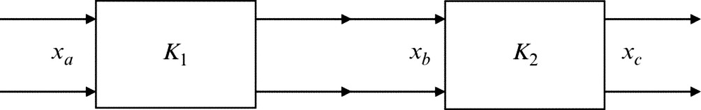
and the equations of the second subnetwork into a similar form
the elimination of internal variables in the interconnected subnetwork is immediate, and the final equations are obtained as
The above equations thus describe the input-output relationship in the cascade connection.
If one writes Eq. (6.20) explicitly into

the output vector xb (with a sign change in ib) of Eq. (6.23) is the input vector to a second subnetwork in cascade with the first. The matrix K appearing in Eq. (6.23) is naturally called the chain matrix of the 2n-port, and one has the following theorem.
The above cascade structure is the most salient characteristic feature of the chain matrix. In terms of control, the chain matrix represents the feedback simply as a multiplication of a matrix. This property makes the analysis of closed-loop systems very simple and makes the role of factorization clearer. Based on this, Kimura [22] brought forward the use of chain-scattering matrix in control system design. Another remarkable property of the CSR is the symmetry (duality) between the CSR and its inverse. This property is also regarded to be quite relevant to control system design.
A serious disadvantage of the CSR is, however, that it only exists for the special plants that satisfy certain full rank conditions. In order to obtain the CSR of the general plants that do not satisfy the full rank conditions, one is forced to augment the plants. Such augmentation is, however, irrelevant to and has no implication in control system design.
This book will present a generalization of the CSR to the case of general plants. Through the notion of input-output consistency, the conditions under which the generalized CSR and the dual generalized CSR exist will be proposed. The generalized chain-scattering matrices will be formulated into a general parameterized form by using the generalized inverse of matrices. The algebraic system properties such as the cascade structure and the symmetry (duality) property of this approach will be exploited completely.
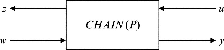
Consider a plant P (Fig. 6.3) with two kinds of inputs (w, u) and two kinds of outputs (z, y) represented by


where Pij (i, j = 1, 2) are all rational matrices with dimensions mi × kj (i, j = 1, 2).
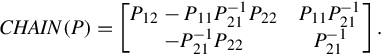
If P21 is invertible, then one has the CSR of P as
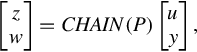
where
If P represents a usual input-output relation of a system, CHAIN(P) represents the characteristic of power ports which in turn reflects physical structure of the plant. The CSR describes the plant as a wave scatterer between (u, z)-wave and the (w, y)-wave that travel oppositely to each other (Fig. 6.4).
The main reason of using the CSR lies in its ability to represent the feedback connection as a cascade one. The cascade connection of two CSRs, G1 and G2, is actually a feedback connection because the loops across the two systems, G1 and G2, exists. The resulting CSR is just G1G2 of the two representation. This property thus greatly simplifies the analysis and synthesis of feedback connection. This can be seen by eliminating the intermediate variables (z1, w1) from the following relations:

If Gi = CHAIN(Pi), i = 1, 2, the cascade connection represents the feedback connection represented in Fig. 6.5. This connection is also termed a star product in Redheffer [91]. The use of CSR simply represents this connection by the product of the two individual representations.

Another interesting property of CSR is that its inverse (if exists) is dually represented as
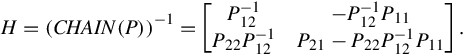
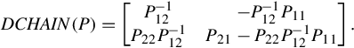
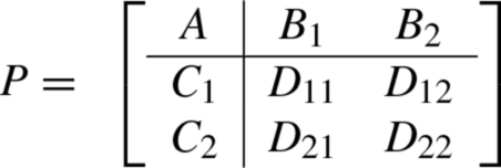
The representation (6.28) exists if P12 is invertible. It is called the dual CSR of P which is denoted by
The duality between CHAIN(P) and DCHAIN(P) is represented in the following identity

Now, we look at the realizations of the CSR and the dual CSRs. Let
 (6.31)
be a state-space realization of the plant P. In order to obtain the realization of the CSR and the dual CSRs, one may write out the following state equation of the plant P explicitly
In order that state space representations of CHAIN(P) and DCHAIN(P) exist, one must assume that ![]() and
and ![]() exist. In that case, one can solve Eq. (6.34) for w yielding
exist. In that case, one can solve Eq. (6.34) for w yielding
By substituting this relation into Eqs. (6.32), (6.33), one has a realization of CHAIN(P) as
 (6.36)
Similarly, DCHAIN(P) is given by
 (6.37)
6.4 Conclusions
This chapter has briefly introduced certain fundamental approaches to control system analysis, specifically the PMD theory, the behavioral approach and the CSR. Based on these, this book will present its main contributions in the following chapters. In the PMD theory, our interests will be focused on certain fundamental issues as determination of the finite and infinite frequency structure of any rational matrix, analysis of the resolvent decomposition of a regular polynomial matrix and formulations of the solution of a regular PMD.
Concerning the chain-scattering representation, this book will provide a generalization to the known approach. Such a generalized CSR is believed to be useful in circuit theory and ![]() control theory. Related to the behavior theory, this book will present a new notion: realization of behavior. Realization of behavior is seen to be a converse procedure to the latent variable elimination theorem [27]. Finally, two key notions in control system analysis, well-posedness and internal stability, will be discussed.
control theory. Related to the behavior theory, this book will present a new notion: realization of behavior. Realization of behavior is seen to be a converse procedure to the latent variable elimination theorem [27]. Finally, two key notions in control system analysis, well-posedness and internal stability, will be discussed.