
The solution of a regular PMD and the set of impulsive free initial conditions
Abstract
In this chapter, we discuss the complete solution of the linear nonhomogeneous matrix differential equations. What is meant by the complete solution is the full solution taking into account the initial conditions of the state as well as the initial conditions of the input. The essence of the new results presented here with respect to the existing results is that the obtained solution displays the full solution components including the impulse response and the slow response created, not only by the initial conditions of the state, but also by the initial condition of the input. Special attention is drawn to the initial conditions of the system input. Compared to the known results, in which the initial conditions of the system input are usually assumed to be zero, our approach firstly considers this issue explicitly.
Keywords
Linear nonhomogeneous matrix differential equations (LNHMDEs); Complete solution; Initial conditions; Impulse response; Slow response; Generalized state space systems; Singular perturbation model; Algebraic matrix Riccati equation; Slow state (smooth state); Fast state (impulsive state)
8.1 Introduction
In this chapter, we discuss the complete solution of the linear nonhomogeneous matrix differential equations (LNHMDEs). What is meant by the complete solution is the full solution taking into account the initial conditions of the state as well as the initial conditions of the input. The essence of the new results presented here with respect to the existing results [13, 17, 102] is that the obtained solution displays the full solution components including the impulse response and the slow response created, not only by the initial conditions of the state, but also by the initial condition of the input. Special attention is drawn to the initial conditions of the system input. Compared to the known results [13, 17, 102], in which the initial conditions of the system input are usually assumed to be zero, our approach firstly considers this issue explicitly.
The LNHMDEs or linear nonhomogeneous regular polynomial matrix descriptions (PMDs) are described by
where ρ := d/dt is the differential operator, ![]() , rankR(ρ)A(ρ) = r, Ai ∈ Rr×r, i = 0, 1, 2, …, q1, q1 ≥ 1, B(ρ) = Blρl + Bl−1ρl−1 + ⋯ + B1ρ + B0 ∈ R[ρ]r×m, Bj ∈ Rr×m, j = 0, 1, 2, …, l, l ≥ 0,
, rankR(ρ)A(ρ) = r, Ai ∈ Rr×r, i = 0, 1, 2, …, q1, q1 ≥ 1, B(ρ) = Blρl + Bl−1ρl−1 + ⋯ + B1ρ + B0 ∈ R[ρ]r×m, Bj ∈ Rr×m, j = 0, 1, 2, …, l, l ≥ 0, ![]() is the pseudo-state of the LNHMDE,
is the pseudo-state of the LNHMDE, ![]() is an i times piecewise continuously differentiable function called the input of the LNHMDE. Their homogeneous cases
is an i times piecewise continuously differentiable function called the input of the LNHMDE. Their homogeneous cases
are called the linear homogeneous matrix differential equations (LHMDEs) or homogeneous PMDs. Both regular generalized state space systems (GSSSs), which are described by
where E is a singular matrix, rank(ρE − A) = r, and the (regular) state space systems, which are described by
are special cases of the above LNHMDEs (4.1). There have been many discussions about GSSSs (see, e.g., [7–11, 103, 104]). In [12], the impulsive solution to the LHMDEs was presented in a closed form. For both the LNHMDEs and LHMDEs, Vardulakis [13] developed their solutions under the assumption that both the initial conditions of the state and the input are zero. However, as we will see later, in some real cases, the initial conditions of the state might result from a random disturbance entering the system, and a feedback controller is called for. Since the precise value of the initial conditions of the state is unpredictable and the control is likely to depend on those initial conditions of the state, so this assumption is somewhat stronger than necessary.
Example 8.1.1
This example is to display the fact that the initial conditions of u(t) are not necessarily equal to zero in some situations.
To the singular perturbation model [105]

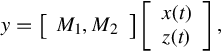
where x(t) ∈ Rn, z(t) ∈ Rm, u(t) ∈ Rr, and y(t) ∈ Rp. Kokotovic et al. [105] considered the so-called near-optimal regulator problem, i.e., to find a control u(t) ∈ Rr, t ≥ 0 so as to regulate the state  to the original by way of minimizing the quadratic performance index
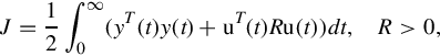
where the r × r weighting matrix R penalizes excessive values of control u(t). The solution of the above problem is the optimal linear feedback control law
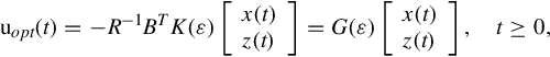
where K(ε) satisfies the algebraic matrix Riccati equation. When the original system satisfies some conditions, K(ε) exist as a positive-definite matrix (see [105, page 111, Theorem 4.1]).
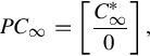
Let us investigate a special case with B1 = In, B2 = Im, and note that the matrix K(ε) is positive-definite, and thus is nonsingular. In this case, the matrix G(ε) is of full column rank. Therefore if

then

In this chapter, we will present a solution to Eq. (8.1) that displays the impulse response and the slow response created not only by the initial conditions of βNH(t), but also by the initial condition of u(t). Also reformulations to the solution of the LNHMDEs in terms of the regular derivatives of u(t) are given. By defining the slow state (smooth state) and the fast state (impulsive state) of them, it is shown that the system behaviors of the LNHMDEs can be decomposed into the slow response (smooth response) and the fast response (impulsive response) completely. This approach is applied conveniently to discuss the impulse free initial conditions of Eq. (8.1).
So far there have been many discussions about the impulse free condition either of the GSSSs (see, e.g., [14, 15]) or of the LNHMDEs and the LNHMDEs (see, e.g., [13, 16]). However, the common concern in the known results is the impulse created by the appropriate initial conditions of the state alone. For LNHMDEs, a different analysis concerning this issue is carried out that considers both the impulse created by the initial conditions of u(t) and that created by the initial conditions of βNH(t).
8.2 Preliminary results
Any rational matrix A(s) is equivalent [87] at ![]() to its Smith-McMillan form, having the form:
to its Smith-McMillan form, having the form:

where 1 ≤ k ≤ r and ![]() Any polynomial matrix
Any polynomial matrix ![]() with
with ![]() can be transformed by unimodular transformation to its Smith form
can be transformed by unimodular transformation to its Smith form
where 1 ≤ k ≤ r, fj(s)/fj+1(s), j = k, k + 1, …, r − 1. We denote ![]() ,
, ![]() , i ∈ I, j = k, k + 1, …, r as the Jordan Chain of lengths σij corresponding to the eigenvalue λi of A(s) and consider matrices
, i ∈ I, j = k, k + 1, …, r as the Jordan Chain of lengths σij corresponding to the eigenvalue λi of A(s) and consider matrices
where ![]() and
and
where ![]() , i ∈ I, j = k, k + 1, …, r, is the Jordan block matrix.
, i ∈ I, j = k, k + 1, …, r, is the Jordan block matrix.
Definition 8.2.2
([13])
The pair: ![]() ,
, ![]() , where
, where

![]() , is called an infinite Jordan pair of A(s) if it is a (finite) Jordan pair of the “dual” polynomial matrix:
, is called an infinite Jordan pair of A(s) if it is a (finite) Jordan pair of the “dual” polynomial matrix: ![]() corresponding to its zero at w = 0.
corresponding to its zero at w = 0.
Theorem 8.2.1
([13])
For a regular matrix polynomial A(s), its inverse matrix A−1(s) can be written
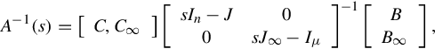
where ![]() where
where ![]() are the orders of the zeros at
are the orders of the zeros at ![]() of A(s).
of A(s).
Proposition 8.2.1
([106])
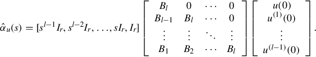
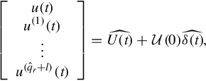
If u(t)(i) denotes the distributional derivative of u(t), u(t)[i] denotes the regular derivative of u(t), δ(t) denotes the impulsive function, then we have the identity

8.3 A solution for the LNHMDEs
To the LNHMDEs
Assuming that the initial values of u(t) and its (l − 1)-derivatives at t = 0 are u(0), u(1)(0)⋯u(l−1)(0) and that the initial values of βNH(t) and its (q1 − 1)-derivatives at t = 0 are ![]() Taking the Laplace transformation of Eq. (8.7), we obtain
Taking the Laplace transformation of Eq. (8.7), we obtain
where ![]() . Because of the Laplace-transformation rule
. Because of the Laplace-transformation rule


![]() can be written [107] as follows
can be written [107] as follows

We denote A−1(s) = Hpol(s) + Hsp(s), where Hpol(s) is the polynomial part of A−1(s) and Hsp(s) is the strictly proper part of A−1(s). To find a minimal realization of Hsp(s)(C, J, B) and a minimal realization of ![]() such that (C, J) and
such that (C, J) and ![]() are a finite Jordan pair and an infinite Jordan pair of A(s), respectively, and
are a finite Jordan pair and an infinite Jordan pair of A(s), respectively, and
We obtain from [13]

where
Similarly,

where

From [13] we also obtain
where

Now Eq. (8.8) can be written as
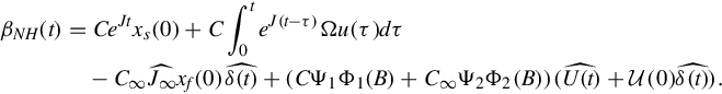
By taking the inverse Laplace transformation of the above, we finally obtain the following theorem that represents the required complete solution of the LNHMDE (8.7) created by the nonzero initial conditions on both the control u(t) and βNH(t).
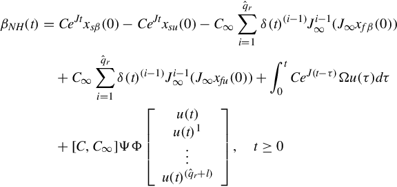
Theorem 8.3.1
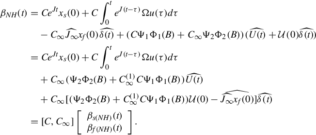
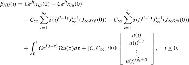
The solution of the LNHMDE (8.7) corresponding to nonzero initial conditions both on the pseudo-state βNH(t) and the input u(t) is

8.4 The smooth and impulsive solution components and impulsive free initial conditions:  is of full row rank
The main aims of this section are to analyze the fast and slow components in the solution of the LNHMDEs and then to characterize the impulsive behavior of the system. To this end, one is suggested to reformulate the solution that is given by Theorem 8.3.1 in terms of the regular derivative of u(t). This is the subject of the following result.
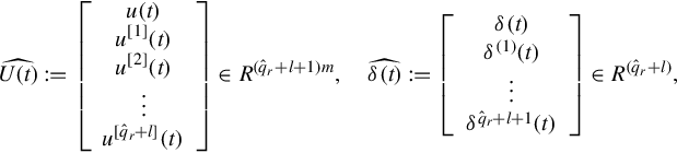
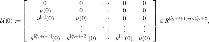
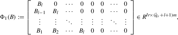
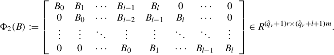
Consider the following notations:
Theorem 8.4.1
With the above notations and assume that ![]() has full row rank and that its {1}-inverse is
has full row rank and that its {1}-inverse is ![]() Denote
Denote
then

Proof
From Eqs. (10.9), (8.12), we know
from Eq. (8.6), we have
if ![]() has full row rank, we have
has full row rank, we have ![]() . Substituting the above into Eq. (10.11), we obtain
. Substituting the above into Eq. (10.11), we obtain
Now we shall generalize the concept of the state to the LNHMDEs as [13] has done for the LHMDEs and the GSSS.
Definition 8.4.1
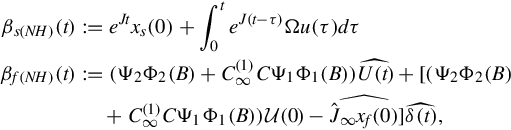
We define the vector
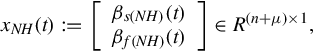
where

as the state of the LNHMDE. βs(NH)(t) is called the slow state or smooth state, βf(NH)(t) is called the fast state or impulsive state.
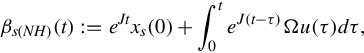
For the LHMDEs
its solution is
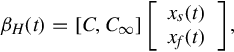
where

It is clear that the impulsive behavior of βH(t) at t = 0 only depends on xf(0), which is only related to the initial conditions of βH(t) and its derivatives at t = 0. Thus the set of impulse free initial conditions for LHMDE A(ρ)βH(t) = 0, t ≥ 0 is [13–16]

However, for the LNHMDEs, this issue becomes much more complicated, for in this case not only the initial conditions of βNH(t), but also the initial conditions of u(t) influence the solution structure. The following result provides an answer to this difficulty.
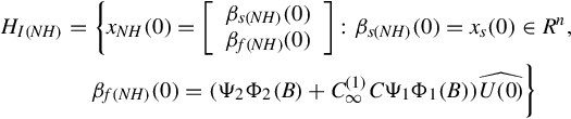
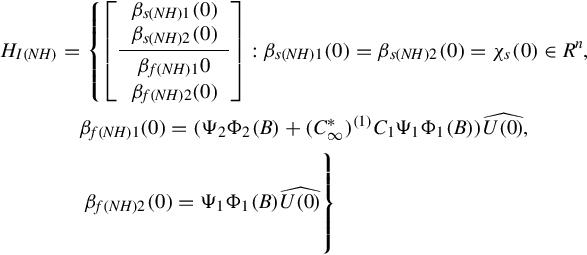
Theorem 8.4.2
Assume that ![]() has full row rank. The set of the impulsive free initial conditions for the LNHMDE (8.7) is
has full row rank. The set of the impulsive free initial conditions for the LNHMDE (8.7) is
Proof
For the LNHMDE (8.7), under the notations in Theorems 8.3.1 and 8.4.1, we partition
where
Observing Eqs. (8.12), (8.13), we can see that βNH(t) is impulse free at t = 0 iff
which hold true iff
i.e.,
and
The set of the impulsive free initial conditions is thus derived from Theorem 8.4.1.

8.5 The smooth and impulsive solution components and impulsive free initial conditions: is not of full row rank
This section is devoted to analyze the solution components and impulsive free initial conditions of the LNHMDEs without assuming that ![]() is of full row rank.
is of full row rank.
If ![]() is not of full row rank, say its row rank is r1 < r, then there exists a transformation called “row compression,” which reduces
is not of full row rank, say its row rank is r1 < r, then there exists a transformation called “row compression,” which reduces ![]() to the form
to the form
where ![]() is of full row rank r1, it thus satisfies
is of full row rank r1, it thus satisfies
If one denotes

where
then one has the following result, which designates the fast and the slow components of the system solution structure.

Proof
From Theorem 8.3.1, one knows that the solution of the LNHMDE (8.7) corresponding to nonzero initial conditions both on the pseudo-state βNH(t) and the input u(t) is
From the Proof of Theorem 8.4.1, one further obtains
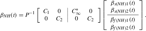
Under the transformation P, the above βNH(t) is seen to be transformed into

where
by the virtue of that ![]() is of full row rank and by using Theorem 8.4.1, the above formulation can subsequently be written into
is of full row rank and by using Theorem 8.4.1, the above formulation can subsequently be written into
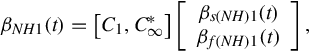
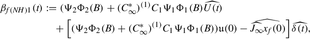
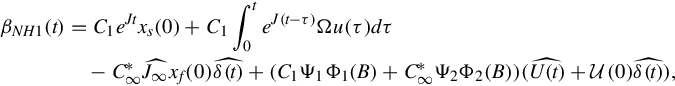
where the components βs(NH)1(t) and βf(NH)1(t) are given by Eqs. (8.22), (8.23), respectively

where the components βs(NH)2(t) and βf(NH)2(t) are given by Eqs. (8.22), (8.24), respectively. By combining Eqs. (8.28), (8.29) and taking the inverse transformation P−1 of Eq. (8.27) one finally establishes the required results.
Remark 8.5.1
The above theorem serves to designate the fast and slow components in the solutions of LNHMDEs in a general setting; it also enables us to analyze the impulse free initial conditions of the systems in the following manner without assuming that ![]() is of full row rank.
is of full row rank.
Proof
From Theorem 8.5.1, it is clearly seen that βNH is impulsive free at t = 0 if and only if βf(NH)1(t) and βf(NH)2(t) are both impulse free at t = 0.
If one partitions
where
Observing Eqs. (8.12), (8.23), one can see that βf(NH)1(t) is impulse free at t = 0 iff
which hold true iff
i.e.,
and
βf(NH)2(t) is impulse free at t = 0, if and only if
The set of the impulsive free initial conditions is thus derived from Theorem 8.5.1.