In this book several contributions to the theory of generalized linear multivariable control are made that provide extensions to some results in polynomial matrix description (PMD) theory, behavioral theory, and ${\mathcal{H}}_{\infty }$ control theory. We highlight the application of linear multivariable control in congestion control of the Internet as well. The remaining parts of this book are organized as follows.

In Chapter 2, we outline the basic components of vector algebra, matrix algebra, linear differential equation, matrix differential equation, and Laplace transform.

Chapter 3 presents a brief introduction of the generalized inverse of matrix, which is needed in the following expositions. This introduction includes the left inverse and right inverse, the Moore-Penrose inverse, the minimization approach to solve an algebraic matrix equation, the full rank decomposition theorem, the least square solution to an algebraic matrix equation, and the singular value decomposition.

The polynomial matrix fraction description (PMFD) is a mathematically efficient and useful representation for a matrix of rational functions. With application to the transfer function of a multiinput, multioutput linear state equation, the PFD can inherit the structural features that, for example, permit natural generalization of minimal realization having established for single-input, single-output state equations. The main aim of Chapter 4 is to lay out a basic introduction to the polynomial fraction description, which is a key mathematical component in the current exposition of the generalized linear multivariable control theory. The main components covered by this chapter are right (left) polynomial fractions, column and row degrees, minimal realization, poles and zeros, and state feedback.

Chapter 5 gives an introduction of the mostly important and basic elements in the stability theory. We surveyed the following theoretical concepts, terms, and statements: internal stability (IS), Lyapunov stability, and input-output stability.

Chapter 6 surveys the fundamental approaches to control system analysis, including the PMD theory of linear multivariable control systems, behavioral approach in systems theory, and the chain-scattering representations (CSR).

The finite and infinite frequency structures of a rational matrix are fundamental to system analysis and design. The classical methods of determining them are not stable in numerical computations, because the methods are based on unimodular matrix transformations that result in an extraordinarily large number of polynomial manipulations. Van Dooren et al. [1] presented a method for determining the Smith-McMillan form of a rational matrix from its Laurent expansion about a particular finite point s₀ ∈ C. Subsequently, Verghese and Kailath [2] and Pugh et al. [3] extended this theory to produce a method of determining the infinite pole and zero structures of a rational matrix from its Laurent expansion about the point at infinity. The difficulty inherent in these approaches is the computation of the Laurent expansion of the original rational matrix, one is forced to calculate all the coefficient matrices in the Laurent expansion; furthermore there is no explicit stop criterion for recursion available in these approaches.

In Chapter 7 a novel method is developed that determines the finite and infinite frequency structure of any rational matrix. For a polynomial matrix, a natural relationship between the rank information of the Toeplitz matrices and the number of the corresponding irreducible elementary divisors (IREDs) in its Smith form is established. This relationship proves to be fundamental and efficient to the study of the finite frequency structure of a polynomial matrix. For a rational matrix, this technique can be employed to find its infinite frequency structure by examining the finite frequency structure of the dual of its companion polynomial matrix. It can also be extended to find the finite frequency structure of a rational matrix via a PMFD. It is neat and numerically stable when compared with the cumbersome and unstable classical procedures based on elementary transformations with unimodular matrices. Compared to the methods of Van Dooren et al. [1], Verghese and Kailath [2], and Pugh et al. [3], our approach, which is based on analyzing the nullity of the Toeplitz matrices of the derivatives of the polynomial matrices rather than the Laurent expansion of the original rational matrices, will be more straightforward and much simpler, for it is easier and more direct to obtain the derivatives of a polynomial matrix than to obtain its Laurent expansion. The special Toeplitz matrices, which are based on the information of the Smith zeros [4, 5] of the system, are relatively easy to compute due to the fact that several numerical algorithms [6] have been proposed for finding the locations of the Smith zeros. Moreover, the procedure will terminate after a minimal number of steps, which thus represents another numerical refinement.

In Chapters 8–10, several contributions are presented concerning the solution of regular PMD.

Chapter 8 considers regular PMDs or linear nonhomogeneous matrix differential equations (LNHMDEs), which are described by

$\begin{array}{l}\hfill A(\rho )\beta (t)=B(\rho )u(t),t\ge 0,\end{array}$

where ρ := d/dt is the differential operator, A(ρ) = A_qρ^q + A_q−1ρ^q−1 + ⋯ + A₁ρ + A₀ ∈ R[ρ]^r×r, rank_R[ρ]A(ρ) = r, A_i ∈ R^r×r, i = 0, 1, 2, …, q, q ≥ 1, B(ρ) = B_lρ^l + B_l−1ρ^l−1 + ⋯ + B_lρ + B₀ ∈ R[ρ]^r×m, B_j ∈ R^r×m, j = 0, 1, 2, …, l, l ≥ 0, $\beta (t):[0,+\infty )\to R^r$ is the pseudo-state of the PMDs, $u(t):[0,+\infty )\to R^m$ is a p times piecewise continuously differentiable function called the input of the PMD. Its homogeneous case

$\begin{array}{l}\hfill A(\rho )\beta (t)=0,t\ge 0\end{array}$

is called the homogeneous PMD or the linear homogeneous matrix differential equations (LHMDEs). Both the regular generalized state space systems (GSSSs), which are described by

$\begin{array}{l}\hfill E\stackrel{.}{x}=Ax(t)+Bu(t),\end{array}$

where E is a singular matrix, rank (ρE − A) = r, and the (regular) state space systems, which are described by

$\begin{array}{l}\hfill \stackrel{.}{x}=Ax(t)+Bu(t)\end{array}$

are special cases of the regular PMDs (Eq. 1.1).

Regarding the solutions of the GSSSs, there have been many discussions [7–11]. In [12], the impulsive solution to the LHMDEs was presented in a closed form. For both the regular PMDs either in homogeneous cases or in nonhomogeneous cases, Vardulakis [13] developed their solutions under the assumption that both the initial conditions of the state and the input are zero. However, as we will see later, in some cases, the initial conditions of the state might result from a random disturbance entering the system, and a feedback controller is called for. Since the precise value of the initial conditions of the state is unpredictable and the control is likely to depend on those initial conditions of the state, so the assumption of zero initial conditions is somewhat stronger than necessary.

In this book, based on any resolvent decomposition of A(s) we will present a complete solution to Eq. (1.1) that displays the impulse response and the slow response created not only by the initial conditions of β(t), but also by the initial condition of u(t). Also a reformulation to the solution of the regular PMDs in terms of the regular derivativesof u(t) is given. By defining the slow state (smooth state) and the fast state (impulsive state) of the solution components, it is shown that the system behaviors of the regular PMDs can be decomposed into theslow response (smooth response) and the fast response (impulsive response) completely. This approach is conveniently applied to discuss the impulse free initial conditions of Eq. (1.1).

So far there have been many discussions about the impulse free initial condition either to the generalized state space systems [14, 15] or to the regular PMDs [13, 16]. However, the common concern in the known results is the impulse created by the appropriate initial conditions of the state alone. To the regular PMDs, a different analysis concerning this issue will be carried out in this book that considers both the impulse created by the initial conditions of u(t) and that which is created by the initial conditions of β(t).

The solution of the above PMDs is generally proposed on the basis of any resolvent decomposition of A(s) given by

$\begin{array}{l}\hfill A^{-1}(s)=C{(s{I}_n-J)}^{-1}Z+C_{\infty }{(s{J}_{\infty }-I_{\epsilon })}^{-1}{Z}_{\infty },\end{array}$

where (C, J) is the finite Jordan pair of A(s), and $(C_{\infty },J_{\infty })$ is the infinite Jordan pair [13, 17] of A(s). Such resolvent decompositions are not unique, but play an important role in formulating the solution of the regular PMDs. The difficulties in the problem of obtaining the solution of the PMD are specific to the particular resolvent decomposition used. From a computation point of view, when the matrices in Eq. (1.3) are of minimal dimensions, it is obviously easiest to obtain the inverse matrix of A(s).

For Eq. (1.1) Gohberg et al. [17] proposed a particular resolvent decomposition, and the solution of it was formulated according to this decomposition. However, the impulsive property of the system at t = 0 was not fully considered in this work. One advantage of this resolvent decomposition however is that it is constructive, due to the fact that the matrices $Z,Z_{\infty }$ in Eq. (1.3) are formulated in terms of the finite and the infinite Jordan pairs. On the other hand in this resolvent decomposition, there appears certain redundant information, in that the dimensions of the infinite Jordan pair are much larger than is actually necessary, which in turn brings some inconvenience in computing the inverse matrix of A(s). In fact some of the infinite elementary divisors [18] that correspond to the infinite poles of A(s) and actually contribute nothing to the solution. Thus the resolvent decomposition can be proposed in a simpler form that has the advantage of giving a more precise insight into the system structure and bringing some convenience in actual computation. Vardulakis [13] obtained a general solution of Eq. (1.1) under the assumption that the initial conditions of ξ(t) are zero. The main idea of this approach is to find the minimal realizations of the strictly proper part and the polynomial part of A⁻¹(s) and then to obtain the required resolvent decomposition. Although this procedure does give good insight into the system structure, the realization approach is not so straightforward by itself and it is consequently more difficult to be applied in actual computation. Furthermore, in this procedure, no explicit formula for Z and $Z_{\infty }$ is available. Apparently, differences arise between the solution of Gohberg et al. [17] and that of Vardulakis [13] due to the fact that these two solutions are expressed through two different resolvent decompositions. Although it is found that the redundant information contained in the solution of Gohberg et al. [17] can be decoupled, an overly large resolvent decomposition definitely brings some inconvenience to actual computation.

One of the main purposes of Chapter 9 is to present a resolvent decomposition, which is a refinement of both results obtained by Gohberg et al. [17] and Vardulakis [13]. It is formulated in terms of the notions of the finite Jordan pairs, infinite Jordan pairs and the generalized infinite Jordan pairs that were defined by Gohberg et al. [17] and Vardulakis [13]. We make clear the issue of infinite Jordan pair noted by Gohberg et al. [17] and Vardulakis [13]. This refined resolvent decomposition captures the essential feature of the system structure. Further, the redundant information that is included in the resolvent decomposition of Gohberg et al. [17] is deleted through a certain transformation, thus the resulting resolvent decomposition inherits the advantages of both the results of Gohberg et al. [17] and of Vardulakis [13]. This refined resolvent decomposition facilitates computation of the inverse matrix of A(s) due to that the dimensions of the matrices used are of minimal.

Based on this proposed resolvent decomposition, a complete solution of a PMD follows that reflects the detailed structure of the zero state response and the zero input response of the system. The complete impulsive properties of the system are also displayed in our solution. Such impulsive properties are not completely displayed in the solution of Gohberg et al. [17]. Although for the homogeneous case this problem is considered in Vardulakis [13], such complete impulsive properties of the system for the general nonhomogeneous regular PMD is not available from Vardulakis [13].

The known solutions are all based on the resolvent decomposition [13, 17] of the regular polynomial matrix A(s), which is formulated in terms of the finite Jordan pairs and the infinite Jordan pairs of A(s). On the one hand, such treatments have the immediate advantage that they separate the system behavior into the slow (smooth) response and the fast (impulsive) response, which may provide a deep insight into the system structure. On the other hand, such treatments bring some inconvenience for the actual computation since the classical methods of determining the finite Jordan pairs or the infinite Jordan pairs have to transform the polynomial matrix A(s) into its Smith-McMillan form or its Smith-McMillan form at infinity. Such transformations are well known not to be stable in numerical computation terms, for they result in an extraordinarily large number of polynomial manipulations.

In Chapter 10 a novel approach via linearization is also presented to determine the complete solution of regular PMDs that takes into account not only the initial conditions on β(t), but also the initial conditions on u(t). One kind of linearization [17] of the regular polynomial matrix A(s) is the so-called generalized companion matrix, which is in fact a regular matrix pencil. The Weierstrass canonical form of this matrix pencil can easily be obtained by certain constant matrix transformations [5]. In this book certain additional properties of this companion form are established, and a special resolvent decompositionof A(s) is proposed that is based on the Weierstrass canonical form of this generalized companion matrix. The solution of the regular PMD is then formulated from this resolvent decomposition. An obvious advantage of the approach adopted here is that it immediately avoids the polynomial matrix transformations necessary to obtain the finite and infinite Jordan pairs of A(s), and only requires the constant matrix transformation to obtain the Weierstrass canonical form of the generalized companion form, which is less sensitive than the former in computational terms. Since numerically efficient algorithms to generate the canonical form of a matrix pencil are well developed [19, 20], the formula proposed here is more attractive in computational terms than the previously known results.

One of the fundamental problems treated in this book originates from classical network theory, where a circuit representation called the chain matrix [21] has been widely used to deal with the cascade connection of circuits arising in analysis and synthesis problems. Recently, Kimura [22] has developed the CSR, which was subsequently used to provide a unified framework for $H^{\infty }$ control theory. The CSR is in fact an alternative way of representing a plant. Compared to the usual transfer function formulation, it has some remarkable properties. One is its cascade structure, which enables feedback to be represented as a matrix multiplication. The other is the symmetry (duality) between the CSR and its inverse called the dual chain-scattering representation (DCSR). Due to these characteristic features, it has successfully been used in several areas of control system design [22–24].

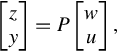
Consider a plant P with two kinds of inputs (w, u) and two kinds of outputs (z, y) represented by

$\begin{array}{l}\hfill \left[\begin{array}{l}\hfill z\hfill \\ \hfill y\hfill \end{array}\right]=P\left[\begin{array}{l}\hfill w\hfill \\ \hfill u\hfill \end{array}\right]=\left[\begin{array}{ll}\hfill P_{11}\hfill & \hfill P_{12}\hfill \\ \hfill P_{21}\hfill & \hfill P_{22}\hfill \end{array}\right]\left[\begin{array}{l}\hfill w\hfill \\ \hfill u\hfill \end{array}\right],\end{array}$

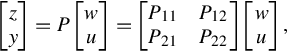
where P_ij (i = 1, 2; j = 1, 2) are all rational matrices with dimensions m_i × k_j (i = 1, 2; j = 1, 2). In order to compute the CSR and DCSR of Eq. (1.4), P₂₁ and P₁₂ are generally assumed to be invertible [22]. However, for general plants, if neither of P₁₂ and P₂₁ is invertible, one cannot use CSR and DCSR directly. Although the approach was extended by Kimura [22] to the case in which P₁₂ is full column rank and P₂₁ is full row rank by augmenting the plant, a systematic treatment is still needed in the general setting when neither of these conditions is satisfied.

In Chapter 11, we consider general plants, and therefore make no assumption about the rank of P₁₂ and P₂₁. From an input-output consistency point of view, the conditions under which the CSR exist are developed. These conditions essentially relax those assumptions that were generally put on the rank of P₂₁ and P₁₂ and make it possible to extend the applications of the CSR approach from the regular cases of the 1-block case, the 2-block case and the 4-block case [25] to the general case. Based on this, the chain-scattering matrices are formulated into general parameterized forms by using the matrix generalized inverse. Subsequently the cascade structure property and the symmetry are investigated.

Recently, behavioral theory [26, 27] has received broad acceptance as an approach for modeling dynamical systems. One of the main features of the behavioral approach is that it does not use the conventional input-output structure in describing systems. Instead, a mathematical model is used to represent the systems in which the collection of time trajectories of the relevant variables are viewed as the behavior of the dynamical systems. This approach has been shown [26, 28] to be powerful in system modeling and analysis. In contrast to this, the classical theories such as Kalman’s state-space description and Rosenbrock’s PMD take the input-output representation as their starting point. In many control contexts it has proven to be very convenient to adopt the classical input-state-output framework. It is often found that the system models, in many situations, can easily be formulated into the input-state-output models such as the state space descriptions and the PMDs. Based on such input-state-output representations, the action of the controller can usually be explained in a very natural manner and the control aims can usually be attained very effectively.

As far as the issue of system modeling is concerned, the computer-aided procedure, i.e., the automated modeling technology, has been well developed as a practical approach over recent years. If the physical description of a system is known, the automated modeling approach can be applied to find a set of equations to describe the dynamical behavior of the given system. It is seen that, in many cases, such as in an electrical circuit or, more generally, in an interconnection of blocks, such a physical description is more conveniently specified though the frequency domain behavior of the system. Consequently in these cases, a more general theoretic problem arises, i.e., if the frequency domain behavior description of a system is known, what is the corresponding dynamical behavior? In other words, what is the input-output or input-state-output structure in the time domain that generates the given frequency domain description. It turns out that this question can be interpreted through the notion of realization of behavior which we shall introduce in Chapter 12. In fact, as we shall see later, realization of behavior, in many cases, amounts to introduction of latent variables in the time domain. From this point of view, realization of behavior can be understood as a converse procedure to the latent variable elimination theorem [27]. It should be emphasized that realization of behavior also generalizes the notion of transfer function matrix realization in the classical control theory framework, as the behavior equation is a more general description than the transfer function matrix. As a special case, the behavior equations determine a transfer matrix of the system if they represent an input-output system [27, 29], i.e., when the matrices describing the system satisfy a full rank condition.

More recently in [30], a realization approach was suggested that reduces high-order linear differential equations to the first-order system representations by using the method of “linearization.” From the point of view of realization in a physical sense one is, however, forced to start from the system frequency behavior description rather than from the high-order linear differential equations in time domain.

The main aim of Chapter 12 is to present one new notion of realization of behavior. Further to the results of [31]. The input-output structure of the GCSRs and the DGCSRs are thus clarified by using this approach. Subsequently the corresponding autoregressive-moving-average (ARMA) representations are proposed and are proved to be realizations of behavior for any GCSR and for any DGCSR. Once these ARMA representations are proposed, one can further find the corresponding first-order system representations by using the method of Rosenthal and Schumacher [30] or other well-developed realization approaches such as Kailath [32]. These results are interesting in that they provide a good insight into the natural relationship between the (frequency) behavior of any GCSR and any DGCSR and the (dynamical) behavior of the corresponding ARMA representations. Since no numerical computation is involved in this approach, realization of behavior is particularly accessible for the situations in which the coefficients are symbolic rather than numerical.

The process of designing a control system generally involves many steps. There are many issues, most importantly modeling, which need to be considered before a controller is designed. The task in control system design is, therefore, not merely to design control systems for the known plants. It also involves investigating practical models. It is thus important to realize at the outset that some practical problems [33, 34] arising in engineering practice often provide rich information of the system input signals.

Modern ${\mathcal{H}}_{\infty }$ and ${\mathcal{H}}_2$ control theory are powerful tools for control system design. Zames [35] originally formulated the ${\mathcal{H}}_{\infty }$ optimal control problem in an input-output setting. The more recent ${\mathcal{H}}_{\infty }$ control theories ([36, 37], only document two instances) took the standard control feedback configuration (model), on which some standing assumptions are made, as their starting point. Such approaches, capture all the essential features of the general problem and the proposed theories are thus accessible to engineering practice on one hand, but involve some sacrifice of generality on the other hand. Such sacrifice of generality essentially result from the standing assumptions that are made on the system (plant) to achieve system well-posedness (WP) and IS. In some circumstances, these assumptions are not necessarily satisfied by the actual plants [38]. Such sacrifice of generality may also result from the impact of the input signal on the system control design not being included in the consideration.

In this case, it is interesting to consider the relaxations of the general requirements of WP and IS from the point of view of the impact of the input signal information on the system control design, to treat this issue explicitly and to give quantitative and qualitative results about it. This subject is addressed in this book. The input signal information is considered in analyzing the issues that are related to system WP and IS.

Consider the standard feedback configuration given in Fig. 1.1, where P is the plant and K is the controller. The plant accounts for all system components except for the controller. The signal w contains all external inputs, including disturbances, sensor noise, and commands. In some circumstances, the input signal w belongs to a set that can be characterized to some degree [39]. The output z is an error signal, y is the vector of measured variables, and u is the control input. All these signals z, y, w, and u are real rational vectors in the complex variable s = λ + jω. The equations that describe the feedback configuration of Fig. 1.1 are

$\begin{array}{l}\hfill \left[\begin{array}{l}\hfill z\hfill \\ \hfill y\hfill \end{array}\right]=P\left[\begin{array}{l}\hfill w\hfill \\ \hfill u\hfill \end{array}\right],\end{array}$

$\begin{array}{l}\hfill u=Ky,\end{array}$

where P and K are real rational transfer matrices in the complex variable s = λ + jω. This means that only finite-dimensional linear time-invariant systems are considered. We write

$\begin{array}{l}\hfill P=\left[\begin{array}{ll}\hfill P_{11}\hfill & \hfill P_{12}\hfill \\ \hfill P_{21}\hfill & \hfill P_{22}\hfill \end{array}\right],\end{array}$

where the partitioning is consistent with the dimensions of z, y and w, u. These will be denoted respectively by l₁, l₂ and m₁, m₂.

Roughly speaking, ${\mathcal{H}}_{\infty }$ control problem consists of finding a controller that makes the closed-loop system well-posed, have IS and minimizes the ${\mathcal{H}}_{\infty }$ norm of the closed-loop transfer function. The basic requirements in this problem are WP and IS [36, 39, 40]. The so-called WP requirement is that the matrix (I − P₂₂K) (or (I − KP₂₂)) be invertible, while IS guarantees bounded signals z, u, y for all bounded input signals w.

There are various reasons to consider relaxation of these two requirements in some circumstances; in other words, it is necessary to generalize these two classical notions to include some nonregular cases:

• The known approaches in ${\mathcal{H}}_{\infty }$ control theory either in the state space framework [37] or in the frequency domain framework [36] make a number of technical assumptions as to the plant, including certain rank conditions on P₂₁ and P₁₂. These conditions, simplify the problems and make the approaches be more accessible in engineering practice on the one hand and limit the applicability of the standard problem on the other hand, due to the fact that these conditions are indeed irrelevant for control system design [38]. It was seen [38] that, in some actual situations, such as in the minimum sensitivity problem [35], the usual rank assumptions on P₂₁ and P₁₂ are not satisfied.

• In some practical circumstances, the input signal w belongs to a set that can be characterized to some degree [39]. It is frequently known in advance or is measurable on-line. It will be shown later in this book that the known information of the input signal opens possibility of relaxing the standing requirements of WP and IS.

• The ${\mathcal{H}}_{\infty }$ or ${\mathcal{H}}_2$ control problem in fact amounts to the constrained minimization problems. The constraints come from a WP requirement and an IS requirement and the object we seek to minimize is the ${\mathcal{H}}_{\infty }$ norm or ${\mathcal{H}}_2$ norm of the closed-loop transfer function. If these two requirements are relaxed, it will definitely enable us to search the appropriate controllers in a wider area; the resulting controllers might thus be more flexible in accomplishing the control aims. This need is indeed seen from the following situations. The fact that P₁₂ and P₂₁ do not need to have full rank at $\infty$, as usually required, allows the study of the celebrated minimum-sensitivity problem [35]. Also by relaxing the usual requirement that the entire feedback system be stable, the relaxed requirement that K stabilize P₂₂ allows the inclusion unstable weighting filters (including such that have poles on the imaginary axis) in the mixed sensitivity problem [41].

• For some plants, there is no controller that can make the closed-loop systems have IS. There exist, however, controllers to make the input-output transfer function T_{z, w} (from w to z) stable. For such plants, one may still be interested in designing a controller to achieve this input-output stability and also to accomplish other control aims. In this situation, one thus has to relax the IS requirement.

The main aim of Chapter 13 is to present a certain generalization to the classical concepts of WP and IS. The input consistency and output uniqueness of the closed-loop system in the standard control feedback configurations are investigated. Based on this, a number of notions are introduced such as fully internal well-posedness (FIWP), externally internal well-posedness (EIWP), and externally internal stability (EIS), which characterize the rich input-output and stability features of the general control systems in a general setting. It is shown that, FIWP is equivalent to the classical assumption WP, which has been widely adopted in control system designs, while EIWP and EIS generalize the notions of WP and IS. Some conditions are established to verify EIWP by using the approach of the generalized matrix inverses. Natural links between EIWP and WP, EIS and IS are pointed out. This approach also leads to a generalization of the linear fractional transformation (LFT). The generalized linear fractional transformations (GLFTs) are formulated into some general parameterized forms by using the generalized inverse of matrices. Finally, on the basis of these notions of EIWP, EIS, and GLFT, the extended ${\mathcal{H}}_{\infty }$ control problem is defined in a general setting.

The nonstandard $H_{\infty }$ control problem is the case where the direct feedthroughs from the input to the error and from the exogenous signal to the output are not necessarily of full rank. This problem is reformulated based on the generalized chain-scattering representation (GCSR) in Chapter 14. The GCSR approach leads naturally to a generalization of the homographic transformation. The state-space realization for this generalized homographic transformation and a number of fundamental cascade structures of the $H_{\infty }$ control systems are further studied in a unified framework of GCSR. Certain sufficient conditions for the solvability of the nonstandard $H_{\infty }$ control problem are therefore established via a ($J,J^{\prime }$)-lossless factorization of GCSR. These results present extensions to Kimura’s results on the CSR approach to the $H_{\infty }$ control in the standard case.

The working mechanism of today’s Internet is a feedback system, with the responsibility of managing the allocation of bandwidth resources between competing traffic flows and control the congestion. Congestion control mechanisms in the Internet represent one of the largest deployed artificial feedback systems [42]. The main aim of Chapter 15 is to give an outline of the Internet congestion control from the perspective of linear multivariable control system. We bring this subject into a control domain by looking at the transferring relations between the dynamics of individual flow rates and the dynamics of aggregate flow rates, the transferring relations between link price and flow aggregate price from a multivariable control point of views including the Smith-McMillan forms. Finally we look at the issue of feedback control design to relate the TCP source flow rate with the aggregate flow price, which is in a proportional (P) controller structure. These analyses in the flow level then constitute a theoretical basis for TCP protocol design in the packet level.

We now summarize the key components of the current book: Chapters 2 through 5 covers the mathematical preliminaries and the basic background in linear control systems. Chapter 6 presents an introduction to such fundamental theories on control system structure and behavior as the PMD theory, the CSR approaches, the behavioral theory, and ${\mathcal{H}}_{\infty }$ control theory. Chapter 7 gives a novel method to determine the finite and infinite frequency structure of a rational matrix. Chapters 8–10 are devoted to the resolvent decomposition of a regular polynomial matrix and the solution of regular PMDs. A generalization to the CSR for general plants is presented in Chapter 11. A new notion realization of behavior and its applications are introduced in Chapter 12. Some related extensions to system well-posed-ness and internal stability in ${\mathcal{H}}_{\infty }$ control theory are represented in Chapter 13. Chapter 14 defines and discusses the nonstandard $H_{\infty }$ control problem from a GCSR approach perspective and its solution. Chapter 14 presents applications of linear multivariable control in Internet congestion control. Finally Chapter 16 gives conclusions and some topics for further research.