1.5. Some Important Sample Statistics and Their Distributions

We have already encountered two important sample statistics in the previous section, namely the sample mean vector in Equation 1.1 and the sample variance-covariance matrix S in Equation 1.2. These quantities play a pivotal role in defining the test statistics useful in various hypothesis testing problems. The underlying assumption of multivariate normal population is crucial in obtaining the distribution of these test statistics. Therefore, we will assume that the sample y1, ..., yn of size n is obtained from a multivariate population N_p(μ, Σ).

As we have already indicated, ~ N_p(μ, Σ/n) and (n - 1)S ~ W_p(n - 1, Σ). Consequently, any linear combination of , say c′, c ≠ 0, follows N₁(c′μ, c′Σc/n) and the quadratic form (n - 1)c′Sc/c′Σc ~ χ²(n - 1). Further, as pointed out earlier, and S are independently distributed and hence the quantity follows a t-distribution with (n - 1) degrees of freedom. A useful application of this fact is in testing problems for certain contrasts or in testing problems involving a given linear combination of the components of the mean vector.

Often interest may be in testing a hypothesis if the population has its mean vector equal to a given vector, say μ₀. Since ~ N_p(μ, Σ/n), it follows that z = Σ^−½( - μ) follows N_p(0, I). This implies that the components of z are independent and have the standard normal distribution. As a result, if μ is equal to μ₀ the quantity, z₁² + ... + z_p² = z′z = n( - μ₀)′Σ⁻( - μ₀) follows a chi-square distribution with p degrees of freedom. On the other hand, if μ is not equal to μ₀, then this quantity will not have a chi-square distribution. This observation provides a way of testing the hypothesis that the mean of the normal population is equal to a given vector μ₀. However, the assumption of known Σ is needed to actually perform this test. If Σ is unknown, it seems natural to replace it in n( - μ)′Σ⁻¹( - μ) by its unbiased estimator S, leading to Hotelling's T² test statistic defined as

T² = n( - μ₀)′ S⁻¹( - μ₀),

where we assume that n ≥ p + 1. This assumption ensures that S admits an inverse. Under the hypothesis mentioned above, namely μ = μ₀, the quantity follows an F distribution with degrees of freedom p and n - p.

Assuming normality, the maximum likelihood estimates of μ and Σ are known to be

and

While _ml = is unbiased for μ, _ml = Sn is a (negatively) biased estimator of Σ. These quantities are also needed in the process of deriving various maximum likelihood-based tests for the hypothesis testing problems. In general, to test a hypothesis H₀, the likelihood ratio test based on the maximum likelihood estimates is obtained by first maximizing the likelihood within the parameter space restricted by H₀. The next step is maximizing it over the entire parameter space (that is, by evaluating the likelihood at and ), and then taking the ratio of the two. Thus, the likelihood ratio test statistic can be written as

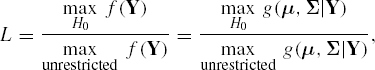
where for optimization purposes the function g(μ, Σ|Y) = f(Y) is viewed as a function of μ and Σ given data Y. A related test statistic is the Wilks' Λ, which is the (2/n)^th power of L. For large n, the quantity −2log L approximately follows a chi-square distribution, with degrees of freedom ν, which is a function of the sample size n, the number of parameters estimated, and the number of restrictions imposed by the parameters involved under H₀.

A detailed discussion of various likelihood ratio tests in multivariate analysis context can be found in Kshirsagar (1972), Muirhead (1982) or in Anderson (1984). A brief review of some of the relevant likelihood ratio tests is given in Chapter 6. There are certain other intuitive statistical tests which have been proposed in various contexts and used in applications instead of the likelihood ratio tests. Some of these tests have been discussed in Chapter 3.