
4.7. Analysis of Covariance
When we want to compare various treatments, but the responses are affected by not only the particular treatments but also by certain other variables termed covariates or concomitant variables, we need to modify the analysis to account for these covariates and eliminate their effects. In other words, to make a fair comparison of various treatments, the data on the response variables need to be made comparable by first adjusting for the covariates. These situations commonly occur in social, biological, medical, physical, and other sciences.
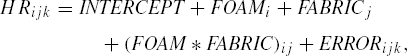
For analyzing these data we utilize the following model
where the matrices Y and ε are defined as before. The term XB represents the design part of the model with a rank of the n by k + 1 matrix X equal to r. The n by q matrix Z is the matrix of data on the covariates with Rank(Z)=q, and the q by p matrix Γ is the matrix of unknown parameters representing the regression of Y on Z. Hence the term ZΓ in the model in Equation 4.7 represents the covariate part of the model. First we want to test the significance of some or all covariates in Z by testing the corresponding rows of Γ to be zero. Second we want to test the linear hypotheses about B, after adjusting for the effects of the variables Z, to answer the usual questions discussed in the earlier sections. We rewrite Equation 4.7 in the standard linear model form as
Then using the usual least squares principle and assuming that the Rank(Z) < n - Rank(X), the least square solutions for Γ and B respectively are
and
where Q = I - X(X′X)-X′.
Now for the first test H0(a) : Γ = 0, that is, covariates have no effect on the response variables, we use the matrices
and
When H0(a) is true, then assuming n > q + r, H and E are independently distributed as Wp(q, Σ) and Wp (n - q - r, Σ) respectively. Using these matrices the usual multivariate tests can be used to test H0(a). Next, for the second test H0(b) : LB = 0, the same E matrix is used and the matrix H is determined using the model
Since H0(b) : LB = 0 can be written as L1Φ = 0 with L1 = (L} : 0), the H matrix for H0(b) is same as that for L1Φ = 0. We use PROC GLM to test these hypotheses, as is illustrated in the next example.
EXAMPLE 7
Comparisons in the Presence of Covariates, A Flammability Study Consider a situation where the interest is in comparing the effects of various types of foams and fabrics used in carpets on carpet flammability. The experiment was designed to determine the most heat-resistant foam and fabric after determining if there were any significant differences between various types of foams and fabrics. The problem appears to fit in the multivariate two-way classification setup. Three types of foams, namely A, B, and C, and three types of fabric materials denoted by X, Y, and Z were used, leading to nine possible compositions for the carpets. Two specimens of equal size (by volume) were taken and separately subjected to flame under identical temperature, pressure, and space. The heat releases at 5, 10, and 15 minutes (HR5, HR10, and HR15) were observed in each experiment.
One important issue, however, needs to be addressed. Although the specimens are all supposedly of the same volume, the amount of heat release relates more to the weight of the specimens than to the volume. Due to different densities for various types of foams and fabrics, the equality of volumes does not necessarily imply the equality of weights of all these specimens. As a result, for a fair comparison, the values of heat releases need to be adjusted for the differing weights of the various specimens. The weight to response relationship does not depend on any other factor. Thus, all effects and contrast tests discussed below are performed at the overall average weight.
These fictitious data inspired by an actual experiment are presented as part of Program 4.7. A two-way classification model with interaction in the classification variables FOAM and FABRIC is fitted for the response variables, HR5, HR10, and HR15. The weight of the specimen (WT) is taken as the covariate.
/* Program 4.7 */
options ls=64 ps=45 nodate nonumber;
    title1 'Output 4.7';
    title2 'Analysis of Covariance';

    data heat ;
    input foam $ fabric $ hr5 hr10 hr15 wt;
    lines ;
    foam_a fabric_x 9.2 18.3 20.4 10.3
    foam_a fabric_x 9.5 17.8 21.1 10.1
    foam_a fabric_y 10.2 15.9 18.9 10.5
    foam_a fabric_y 9.9 16.4  19.2  9.7
    foam_a fabric_Z 7.1 12.8 16.7 9.8
    foam_a fabric_Z 7.3 12.6 16.9 9.9
    foam_b fabric_x 8.2 12.3 15.9 9.5
    foam_b fabric_x 8.0 13.4 15.4 9.3
    foam_b fabric_y 9.4 17.7 21.4 11.0
    foam_b fabric_y 9.9 16.9 21.6 10.8
    foam_b fabric_Z 8.8 14.7 20.1 9.3
    foam_b fabric_Z 8.1 14.1 17.4 7.7
    foam_c fabric_x 7.7 12.5 17.3 10.0
    foam_c fabric_x 7.4 13.3 18.1 10.5
    foam_c fabric_y 8.7 13.9 18.4 9.8
    foam_c fabric_y 8.8 13.5 19.1 9.8
    foam_c fabric_Z 7.7 14.4 18.7 8.5
    foam_c fabric_Z 7.8 15.2 18.1 9.0
    ;
proc glm data = heat;
class foam fabric ;
model hr5 hr10 hr15=wt foam fabric foam*fabric/ss1 nouni;
contrast '(a,z) vs. (c,x)'
intercept 0 foam 1 0 -1 fabric -1 0 1
foam*fabric 0 0 1 0 0 0 -1 0 0 ;
contrast 'foam a vs b ' foam 1 -1 0 ;
manova h = foam fabric foam*fabric/ printe printh ;
run;
/*
proc glm data = heat ;
class foam fabric ;
model hr5 hr10 hr15=wt foam fabric foam*fabric/ss3 nouni;
lsmeans foam fabric foam*fabric ;
contrast 'Foam a vs b ' foam 1 -1 0 ;
contrast '(a,z) vs. (c,x)'
intercept 0 foam 1 0 -1 fabric -1 0 1
foam*fabric 0 0 1 0 0 0 -1 0 0 ;
manova h = foam fabric foam*fabric/ printe printh ;
run;
*/Even though the design appears to be balanced in the variables FOAM and FABRIC, the balancedness is lost due to the presence of the covariate WT as it changes from specimen to specimen. The various types of SS&CP matrices are therefore not identical and a careful analysis of the data is needed.
Since the effects and the SS&CP matrices of the variable FOAM, FABRIC, and FOAM*FABRIC are all to be adjusted for WT, a sequential partitioning of the total SS&CP matrix is appropriate with the WT variable listed first in the corresponding MODEL statement. The partitioning results in all the subsequent SS&CP matrices adjusted at least for this covariate. As far as the other two variables are concerned, there does not appear to be any reason to prefer one over the other. If we want a Type I analysis, we should examine the output resulting from two possible orders in the MODEL statement, namely
model hr5 hr10 hr15 = wt foam fabric foam*fabric/ss1;
and
model hr5 hr10 hr15 = wt fabric foam foam*fabric/ss1;
hoping for consistency in the conclusions. We have, however, chosen to limit our output for the first of these statements.
An examination of Output 4.7 reveals that the interaction FOAM*FABRIC is highly significant under all of the four test criteria. In view of this, it makes sense to conduct various pairwise comparisons for the nine treatments to decide which treatments are similar and which are not. This unfortunately requires as many as 36 pairwise comparisons; in general it is not advisable to perform too many tests since in a large number of pairwise tests, some are likely to appear to be significant just by chance. Based on the least square cell means computed by the LSMEANS statement, it appears that the treatments (A, Z) and (C, X) are comparable with relatively low values for heat release at various time points. The output from the LSMEANS statement is not shown to save space. Suppose we want to see if these two preferred treatments are significantly different from each other. Such a comparison can be made using the CONTRAST statement. Note that the CONTRAST statement should always appear before a MANOVA statement.
Example 4.7. Output 4.7
Analysis of Covariance


         Manova Test Criteria and F Approximations for
        the Hypothesis of no Overall FOAM*FABRIC Effect
H = Type I SS&CP Matrix for FOAM*FABRIC   E = Error SS&CP Matrix

                       S=3    M=0    N=2

Statistic               Value        F    Num DF  Den DF  Pr > F

Wilks' Lambda          0.001717   13.602      12  16.166  0.0001
Pillai's Trace         2.071646   4.4631      12      24  0.0009
Hotelling-Lawley Trace  110.095   42.815      12      14  0.0001
Roy's Greatest Root     107.144   214.29       4       8  0.0001

  NOTE: F Statistic for Roy's Greatest Root is an upper bound.


        Manova Test Criteria and Exact F Statistics for
      the Hypothesis of no Overall (a,z) vs. (c,x) Effect
         H = Contrast SS&CP Matrix for (a,z) vs. (c,x)
                      E = Error SS&CP Matrix

                      S=1    M=0.5    N=2

Statistic               Value        F    Num DF  Den DF  Pr > F

Wilks' Lambda           0.76977   0.5982       3       6  0.6392
Pillai's Trace          0.23023   0.5982       3       6  0.6392
Hotelling-Lawley Trace 0.299089   0.5982       3       6  0.6392
Roy's Greatest Root 0.299089 0.5982 3 6 0.6392 |
In order to identify an appropriate CONTRAST statement, it is helpful to write down the two-way classification model (the covariate term in the model can be ignored for this purpose) for the 1 by 3 response vector HR
where i = A, B, C, j = X, Y, Z and k = 1, 2.
Our interest is in the contrast E(HRAZk - HRCXk), where E indicates the expected value. Dropping the replication suffix 'k' for convenience, this can be written as
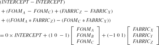

The above representation indicates that in order to get the contrast between treatments (A, Z) and (C, X),
the coefficient for intercept is zero,
the vector of coefficients for the vector of foams (A, B, C)′ is (1 0 -1)′,
the vector of fabrics (X, Y, Z)′ is (-1 0 1)′,
the vector of coefficients for the 9 by 1 vector of interactions
((A*X), (A*Y), (A*Z), (B*X), (B*Y), (B*Z),
(C*X), (C*Y), (C*Z))′
is obtained by respectively putting 1 and −1 at the places corresponding to (A*Z) and (C*X) and zeros elsewhere as follows.
All of this is specified in the CONTRAST statement as
contrast 'label' intercept 0 foam 1 0 -1 fabric -1 0 1
                 foam*fabric 0 0 1 0 0 0 -1 0 0;
The name (A, Z) versus (C, X) enclosed within single quotation marks (' ') in Program 4.7 is used as the label. A label is required in the CONTRAST statement.
For the desired contrast, it is possible to use any of the four multivariate tests. In the present case, since the rank of underlying L matrix is one (there is only a single contrast) all four tests are identical and exact. The corresponding observed value of the F(3, 6) test statistic is 0.5982 leading to a p value of 0.6392. Hence the null hypothesis of no overall difference between (A, Z) and (C, X) treatments cannot be rejected.
Although it is not quite relevant in the present context (because of highly significant interaction), if the interest were to compare the effect of Foam A with that of Foam B, the CONTRAST statement in simplified form could be written as
contrast 'label' foam 1 -1 0;
It is so, since in this case the coefficients of INTERCEPT, the vector of FABRIC, and the vector of FOAM*FABRIC all have zero coefficients and hence need not be explicitly specified in the CONTRAST statement.
Note that in the data presented here, the heat releases at various time points are the repeated measures on the same specimen. Further analysis may be possible using the repeated measures techniques. We address these techniques in Chapters 5 and 6.