1.2. Random Vectors, Means, Variances, and Covariances

Suppose y1,...,y_p are p possibly correlated random variables with respective means (expected values) μ1, ..., μ_p. Let us arrange these random variables as a column vector denoted by y, that is, let

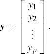
We do the same for μ₁, μ₂, ..., μ_p, and denote the corresponding vector by μ. Then we say that the vector y has the mean μ or in notation E(y) = μ.

Let us denote the covariance between y_i and y_j by σ_ij, i, j = 1, ..., p, that is

σ_ij = cov(y_i, y_j) = E[(y_i - μ_i)(y_j - μ_j)] = E[(y_i - μ_i)y_j] = E(y_iy_j) - μ_iμ_j

and let

Since cov(y_i, y_j) = cov(y_j, y_i), we have σ_ij = σ_ij. Therefore, Σ is symmetric with (i, j)^th and (j, i)^th elements representing the covariance between y_i and y_j. Further, since var(y_i) = cov(y_i, y_i) = σ_ii, the i^th diagonal place of Σ contains the variance of y_i. The matrix Σ is called the dispersion or the variance-covariance matrix of y. In notation, we write this fact as D(y) = Σ. Various books follow alternative notations for D(y) such as cov(y) or var(y). However, we adopt the less ambiguous notation of D(y).

Thus,

Σ = D(y) = E[(y - μ)(y - μ)′] = E[(y - μ)y′] = E(yy′) - μμ′,

where for any matrix (vector) A, the notation A′ represents its transpose.

The quantity tr(Σ) = is called total variance and a determinant of Σ, denoted by |Σ|, is often referred to as the generalized variance. The two are often taken as the overall measures of the variability of the random vector y. However, both of these two measures suffer from certain shortcomings. For example, the total variance tr(Σ) being the sum of only diagonal elements, essentially ignores all covariance terms. On the other hand, the generalized variance |Σ| can be misleading since two very different variance covariance structures can sometimes result in the same value of generalized variance. Johnson and Wichern (1998) provide certain interesting illustrations of such situations.

Let u_p×1 and z_{q × 1} be two random vectors, with respective means μ_u and μ_z. Then the covariance of u with z is defined as

Σ_uz = cov(u, z) = E[(u - μ_u)(z - μ_z)′] = E[(u - μ_u)z′] = E(uz′) - μ_uμ′_z.

Note that as matrices, the p by q matrix Σ_uz = cov(u,z) is not the same as the q by p matrix Σ_zu = cov(z,u), the covariance of z with u. They are, however, related in that

Σ_uz = Σ′_zu.

Notice that for a vector y, cov(y, y) = D(y). Thus, when there is no possibility of confusion, we interchangeably use D(y) and cov(y) (= cov(y, y)) to represent the variance-covariance matrix of y.

A variance-covariance matrix is always positive semidefinite (that is, all its eigenvalues are nonnegative). However, in most of the discussion in this text we encounter dispersion matrices which are positive definite, a condition stronger than positive semidefiniteness in that all eigenvalues are strictly positive. Consequently, such dispersion matrices would also admit an inverse. In the subsequent discussion, we assume our dispersion matrix to be positive definite.

Let us partition the vector y into two subvectors as

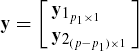
and partition Σ as

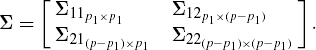
Then, E(y1) = μ₁, E(y2) = μ₂, D(y1) = Σ₁₁, D(y2) = Σ₂₂, cov(y1, y2) = Σ₁₂, cov(y2, y1) = Σ₂₁. We also observe that Σ₁₂ = Σ′₂₁.

The, Pearson's, correlation coefficient, between, y_i, and, y_j, denoted by ρ_ij, is defined by

and accordingly, we define the correlation coefficient matrix of y as

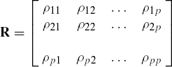
It is easy to verify that the correlation coefficient matrix R is a symmetric positive definite matrix in which all the diagonal elements are unity. The matrix R can be written, in terms of matrix Σ, as

where diag (Σ) is the diagonal matrix obtained by retaining the diagonal elements of Σ and by replacing all the nondiagonal elements by zero. Further, the square root of any matrix A, denoted by A, is a symmetric matrix satisfying the condition, A = AA.

The probability distribution (density) of a vector y, denoted by f(y), is the same as the joint probability distribution of y1, ..., y_p. The marginal distribution f1(y1) of y1 = (y1, ..., y_p1)′, a subvector of y, is obtained by integrating out y2 = (y_p1+1, ..., y_p)′ from the density f(y). The conditional distribution of y2, when y1 has been held fixed, is denoted by g(y2|y1) and is given by

g(y₂|y₁) = f(y)f₁(y₁).

An important concept arising from conditional distribution is the partial correlation coefficient. If we partition y as (y′₁, y′₂)′ where y₁ is a p₁ by 1 vector and y₂ is a (p - p₁) by 1 vector, then the partial correlation coefficient between two components of y₁, say y_i and y_j, is defined as the Pearson's correlation coefficient between y_i and y_j conditional on y₂ (that is, for a given y₂). If Σ_11·2 = (a_ij) is the p₁ by p₁ variance-covariance matrix of y₁ given y₂, then the population partial correlation coefficient between y_i and y_j, i, j = 1, ..., p₁ is given by

The matrix of all partial correlation coefficients ρ_{ij, p1}+1, ..., _p,i, j = 1, ..., p₁ is denoted by R_11·2. More simply, using the matrix notations, R_11·2 can be computed as

[diag (Σ_11·2)]^−½Σ_11·2[diag,(Σ_11·2)]^−½,

where diag, (Σ_11·2) is a diagonal matrix with respective diagonal entries the same as those in Σ_11·2.

Many times it is of interest to find the correlation coefficients between y_i and y_j, i, j = 1, ..., p, conditional on all y_k, k = 1, ..., p, k ≠ i, k ≠ j. In this case, the partial correlation between y_i and y_j can be interpreted as the strength of correlation between the two variables after eliminating the effects of all the remaining variables.

In many linear model situations, we would like to examine the overall association of a set of variables with a given variable. This is often done by finding the correlation between the variable and a particular linear combination of other variables. The Multiple correlation coefficient is an index measuring the association between a random variable y₁ and the set of remaining variables represented by a (p - 1) by 1 vector y₂. It is defined as the maximum correlation between y₁ and c′y₂, a linear combination of y₂, where the maximum is taken over all possible nonzero vectors c. This maximum value, representing the multiple correlation coefficient between y₁ and y₂, is given by

where

and the maximum is attained for the choice c = Σ₂₂⁻¹Σ₂₁. The multiple correlation coefficient always lies between zero and one. The square of the multiple correlation coefficient, often referred to as the population coefficient of determination, is generally used to indicate the power of prediction or the effect of regression.

The concept of multiple correlation can be extended to the case in which the random variable y₁ is replaced by a random vector. This leads to what are called canonical correlation coefficients.