
3.8. General Linear Hypotheses
Sometimes our interest may be in comparing the regression coefficients from the models corresponding to different variables. For example, in a multivariate linear model with two response variables, it may be interesting to test if the intercepts, means, or some other regression coefficients are equal in the respective models corresponding to these two response variables. Such a hypothesis cannot be expressed in the form of Equation 3.11. This hypothesis can, however, be formulated as a general linear hypothesis which can be written as
H0: LBM=0 vs. H1: LBM ≠0,
where r by (k+1) matrix L is, as earlier, of rank r and the p by s matrix M is of rank s. These two matrices have different roles to play and need to be chosen carefully depending on the particular hypothesis to be tested. Specifically, the premultiplied matrix L is used to obtain a linear function of the regression coefficients within the individual models while the postmultiplied matrix M does the same for the coefficients from different models but corresponding to the same set of regressors or independent variables. In other words, the matrix L provides a means of comparison of coefficients within models, whereas the matrix M offers a way for "between models" comparisons of regression coefficients. As a result, the simultaneous pre- and postmultiplication to B by L and M respectively provides a method for defining a general linear hypothesis involving various coefficients of B.
For example, let B = (βij), that is, except for the zeroth row of β, the coefficient βij is the regression coefficient of the ith independent variable in the jth model (that is, the model for jth dependent variable). The zeroth row of β contains intercepts of various models. Suppose we want to test the hypothesis that the difference between the coefficients of first and second independent variables is the same for the two univariate models involving the first two dependent variables. In other words, the null hypothesis to be tested is β11 − β21 = β12 − β22, i.e., H0: (β11 − β21) −(β12 − β22) = 0. This equation in matrix notation is written as LBM=0 with
L= (0 1 − 1 0 ... 0)
and
These types of general linear hypotheses occur frequently in the studies of growth curves, repeated measures, and crossover designed data. Chapter 5 covers various examples of these data.
EXAMPLE 6
Spatial Uniformity in Semiconductor Processes Guo and Sachs (1993) presented a case study that attempted to model and optimize the spatial uniformity of the product output characteristics at different locations in a batch of products. This example empirically models these responses using the multiple response surfaces and interprets the problem of testing the spatial uniformity as a problem of general linear hypothesis testing.
The independent variables under consideration are two flow rates denoted by X1 and X2, and the resulting dependent variables are the deposition rates at three measurement sites. We denote these by y1, y2, and y3 respectively. We are interested in the spatial uniformity, that is, we want to achieve a uniformity between the values of y1, y2, and y3 for the given levels of two flow rates.
This example fits the multivariate regression model for y1, y2, and y3 in terms of X1 and X2. Assume that there is no interaction between X1 and X2 and that the effects of X1 and X2 are both linear. The individual models can be obtained by using the SAS statements
proc reg;
model y1 y2 y3 = x1 x2;
given as part of Program 3.7. Output 3.7, which is produced by Program 3.7, provides the estimates (collected from three separate univariate analyses) of regression coefficients

and hence the three models are
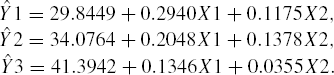
In the ideal case of complete spatial uniformity, we would expect the models for y1, y2, and y3 to be identical. We construct an appropriate null hypothesis from this interpretation of spatial uniformity.
/* Program 3.7 */
options ls=64 ps=45 nodate nonumber;
    data semicond;
    input x1 x2 y1 y2 y3;
    z1=y1−y2;z2=y2−y3;
    lines;
    46 22 45.994 46.296 48.589
    56 22 48.843 48.731 49.681
    66 22 51.555 50.544 50.908
    46 32 47.647 47.846 48.519
    56 32 50.208 49.930 50.072
    66 32 52.931 52.387 51.505
    46 42 47.641 49.488 48.947
    56 42 51.365 51.365 50.642
    66 42 54.436 52.985 51.716
    ;
    /* Source: Guo and Sachs (1993).  Reprinted by permission of the
       Institute of Electrical and Electronics Engineers, Inc.
       Copyright 1993 IEEE. */
    proc reg data = semicond ;
    model y1 y2 y3 =  x1 x2 ;
    AllCoef: mtest y1−y2,y2−y3,intercept,x1,x2/print;
    X1andX2: mtest y1−y2,y2−y3,x1,x2/print;
    title1 ' Output 3.7 ';
    title2 'Spatial Uniformity in Semiconductor Processes' ;
    run;
Let

Then the columns of B represent the regression coefficients in the models for y1, y2, and y3 respectively. Thus the complete spatial uniformity amounts to testing the hypothesis that the three columns of B are identical, that is, our null hypothesis is
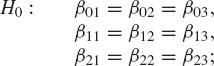
or,

or,
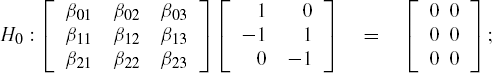
or,

To test this null hypothesis, we use the MTEST statement in PROC REG. An alternative could be to use the CONTRAST and MANOVA statements in PROC GLM, but since that is applicable only for designed experiments and not otherwise, we do not make this choice here. Chapters 4 and 5 elaborate on this approach. The approach using the MTEST statement is general and applicable for all regression modeling problems even when the data are collected from designed or undesigned experiments.
If H0 is true, then the coefficients of the three models are identical. And hence the true means (expected values) of Y1−Y2 and Y2−Y3 would both be zero. Therefore, in order to test H0 we could simultaneously test the three linear hypotheses. Specifically, the null hypotheses are that the intercepts, as well as the coefficients of X1 and X2 in the models for these two variables, are all zero. This can be done using the MTEST statement after the MODEL statement. Models without intercepts can be fitted by using the NOINT option in the MODEL statement.
Consequently, to test H0: LBM=0 with the choice of L and M indicated above, we use the following SAS statements:
proc reg;
model y1 y2 y3 = x1 x2;
mtest y1−y2, y2−y3, intercept, x1, x2/print;
Note that the MTEST statement performs the four multivariate tests on variables Y1−Y2 and Y2−Y3. An alternative yet equivalent approach would have been to define Z1 = Y1− Y2 and Z2 = Y2−Y3 early in the DATA step after INPUT statement as shown below:
data semicond;
input x1 x2 y1 y2 y3;
z1=y1−y2;
z2=y2−y3;
and then later in REG procedure use the MODEL and MTEST statements
model z1 z2 = x1 x2;
mtest z1, z2, intercept, x1, x2/print;
In fact, we do not really need to include variables Z1 and Z2 in the MTEST statement given above. They are included by default because, if the list in the MTEST statement does not include any dependent variable, SAS automatically includes the variables being analyzed and those listed on the left side of the MODEL statement. In Program 3.7 we have, however, used the MTEST statement to avoid creating two extra variables Z1 and Z2. The PRINT option in the MTEST statement prints the corresponding H and E matrices for variables Y1−Y2 and Y2−Y3.
Example 3.7. Output 3.7
Spatial Uniformity in Semiconductor Processes

Model: MODEL1
Dependent Variable: Y1


                      Analysis of Variance

                         Sum of         Mean
Source          DF      Squares       Square      F Value
Prob>F
Model 2 60.14535 30.07268 201.946
0.0001
Error 6 0.89348 0.14891
C Total 8 61.03883
Root MSE 0.38589 R-square 0.9854
Dep Mean 50.06889 Adj R-sq 0.9805
C.V. 0.77073
Parameter Estimates
Parameter Standard T for H0:
Variable DF Estimate Error Parameter=0
INTERCEP 1 29.844889 1.02421553 29.139
X1 1 0.294000 0.01575405 18.662
X2 1 0.117500 0.01575405 7.458
Variable DF Prob > |T|
INTERCEP 1 0.0001
X1 1 0.0001
X2 1 0.0003
Dependent Variable: Y2
Analysis of Variance
Sum of Mean
Source DF Squares Square F Value
Prob>F
Model 2 36.54818 18.27409 251.850
0.0001
Error 6 0.43536 0.07256
C Total 8 36.98354
Root MSE 0.26937 R-square 0.9882
Dep Mean 49.95244 Adj R-sq 0.9843
C.V. 0.53925
Parameter Estimates
Parameter Standard T for H0:
Variable DF Estimate Error Parameter=0
INTERCEP 1 34.076444 0.71494183 47.663
X1 1 0.204767 0.01099694 18.620
X2 1 0.137783 0.01099694 12.529
Variable DF Prob > |T|
INTERCEP 1 0.0001
X1 1 0.0001
X2 1 0.0001
Dependent Variable: Y3Analysis of Variance
Sum of Mean
Source DF Squares Square F Value
Prob>F
Model 2 11.61893 5.80947 183.301
0.0001
Error 6 0.19016 0.03169
C Total 8 11.80910
Root MSE 0.17803 R-square 0.9839
Dep Mean 50.06433 Adj R-sq 0.9785
C.V. 0.35560
Parameter Estimates
Parameter Standard T for H0:
Variable DF Estimate Error Parameter=0
INTERCEP 1 41.394200 0.47250828 87.605
X1 1 0.134567 0.00726792 18.515
X2 1 0.035450 0.00726792 4.878
Variable DF Prob > |T|
INTERCEP 1 0.0001
X1 1 0.0001
X2 1 0.0028
Multivariate Test: ALLCOEF
E, the Error Matrix
1.9090653889 −0.761418778
−0.761418778 0.6168702222
H, the Hypothesis Matrix
5.1464346111 2.3958517778
2.3958517778 9.3527627778
Multivariate Statistics and F Approximations
S=2 M=0 N=1.5
Statistic Value F Num DF Den DF Pr > F
Wilks' Lambda 0.008835 16.064 6 10 0.0001
Pillai's Trace 1.617641 8.4614 6 12 0.0010Hotelling-Lawley Trace 41.27571 27.517 6 8 0.0001
Roy's Greatest Root 39.47972 78.959 3 6 0.0001
NOTE: F Statistic for Roy's Greatest Root is an upper bound.
NOTE: F Statistic for Wilks' Lambda is exact.
Multivariate Test: X1ANDX2
E, the Error Matrix
1.9090653889 −0.761418778
−0.761418778 0.6168702222
H, the Hypothesis Matrix
5.0244008333 2.5131113333
2.5131113333 9.2400906667
Multivariate Statistics and F Approximations
S=2 M=−0.5 N=1.5
Statistic Value F Num DF Den DF Pr > F
Wilks' Lambda 0.00916 23.622 4 10 0.0001
Pillai's Trace 1.605325 12.202 4 12 0.0003
Hotelling-Lawley Trace 41.0887 41.089 4 8 0.0001
Roy's Greatest Root 39.38536 118.16 2 6 0.0001
NOTE: F Statistic for Roy's Greatest Root is an upper bound.
NOTE: F Statistic for Wilks' Lambda is exact. |
The first part of Output 3.7 presents the results of multivariate tests. The error SS&CP matrix E and the hypothesis SS&CP matrix H are given first and are then followed by four multivariate tests. All of the four multivariate tests reject the null hypothesis. For example, the value of Wilks' Λ is 0.0088, which leads to an (exact) F(6,10) statistic value of 16.064 and a p value of 0.0001. In view of this extremely small p value, there is sufficient evidence to reject H0 and conclude the lack of spatial uniformity.
Having rejected the null hypothesis of equality of all regression coefficients including the intercepts in the three models, we may want to test if the three models differ only in their intercepts and if the respective coefficients of X1 and X2 are the same in the models for y1, y2 and y3. Therefore, we exclude the keyword INTERCEPT in the MTEST statement. The appropriate MODEL and MTEST statements are
model y1 y2 y3 =x1 x2;
mtest y1−y2, y2−y3, x1, x2/print;
Of course, as earlier, Y1−Y2 and Y2−Y3 can be removed from the list in the MTEST statement if Z1=Y1−Y2 and Z2 = Y2−Y3 have already been defined in the DATA step and if the variables Z1 and Z2 are analyzed in the MODEL statement. The resulting multivariate outputs would be identical. These are presented under the label, "Multivariate Test: X1ANDX2" in the latter part of Output 3.7. As in the previous case, the null hypothesis in the present case is also rejected by all four multivariate tests leading us to believe that the deposition rates Y1, Y2, and Y3 at the three different measurement sites depend differently on the two flow rates X1 and X2.