
1.6. Tests for Multivariate Normality
Often before doing any statistical modeling, it is crucial to verify if the data at hand satisfy the underlying distributional assumptions. Many times such an examination may be needed for the residuals after fitting various models. For most multivariate analyses, it is thus very important that the data indeed follow the multivariate normal, or if not exactly at least approximately. If the answer to such a query is affirmative, it can often reduce the task of searching for procedures which are robust to the departures from multivariate normality. There are many possibilities for departure from multivariate normality and no single procedure is likely to be robust with respect to all such departures from the multivariate normality assumption. Gnanadesikan (1980) and Mardia (1980) provide excellent reviews of various procedures to verify this assumption.
This assumption is often checked by individually examining the univariate normality through various Q-Q plots or some other plots and can at times be very subjective. One of the relatively simpler and mathematically tractable ways to find a support for the assumption of multivariate normality is by using the tests based on Mardia's multivariate skewness and kurtosis measures. For any general multivariate distribution we define these respectively as
provided that x is independent of y but has the same distribution and
provided that the expectations in the expressions of β1,p and β2,p exist. For the multivariate normal distribution, β1,p = 0 and β2,p = p(p + 2).
For a sample of size n, the estimates of β1,p and β2,p can be obtained as
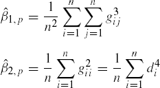
where gij = (yi - ![]() )′Sn−1(yj -
)′Sn−1(yj - ![]() ), and di =
), and di = ![]() is the sample version of the squared Mahalanobis distance (Mahalanobis, 1936) between yi and (μ which is approximated by)
is the sample version of the squared Mahalanobis distance (Mahalanobis, 1936) between yi and (μ which is approximated by) ![]() (Mardia, 1970).
(Mardia, 1970).
The quantity ![]() 1,p (which is the same as the square of sample skewness coefficient when p = 1) as well as
1,p (which is the same as the square of sample skewness coefficient when p = 1) as well as ![]() 2,p (which is the same as the sample kurtosis coefficient when p = 1) are nonnegative. For the multivariate normal data, we would expect
2,p (which is the same as the sample kurtosis coefficient when p = 1) are nonnegative. For the multivariate normal data, we would expect ![]() 1,p to be close to zero. If there is a departure from the spherical symmetry (that is, zero correlation and equal variance),
1,p to be close to zero. If there is a departure from the spherical symmetry (that is, zero correlation and equal variance), ![]() 2,p will be large. The quantity
2,p will be large. The quantity ![]() 2,p is also useful in indicating the extreme behavior in the squared Mahalanobis distance of the observations from the sample mean.
2,p is also useful in indicating the extreme behavior in the squared Mahalanobis distance of the observations from the sample mean.
Thus, ![]() 1,p and
1,p and ![]() 2,p can be utilized to detect departure from multivariate normality. Mardia (1970) has shown that for large samples, κ1 = n
2,p can be utilized to detect departure from multivariate normality. Mardia (1970) has shown that for large samples, κ1 = n![]() 1,p/6 follows a chi-square distribution with degrees of freedom p(p + 1)(p + 2)/6, and κ2 = {
1,p/6 follows a chi-square distribution with degrees of freedom p(p + 1)(p + 2)/6, and κ2 = {![]() 2,p - p(p + 2)}/{8p(p + 2)/n}½ follows a standard normal distribution. Thus, we can use the quantities κ1 and κ2 to test the null hypothesis of multivariate normality. For small n, see the tables for the critical values for these test statistics given by Mardia (1974). He also recommends (Mardia, Kent, and Bibby, 1979, p. 149) that if both the hypotheses are accepted, the normal theory for various tests on the mean vector or the covariance matrix can be used. However, in the presence of nonnormality, the normal theory tests on the mean are sensitive to β1,p, whereas tests on the covariance matrix are influenced by β2,p.
2,p - p(p + 2)}/{8p(p + 2)/n}½ follows a standard normal distribution. Thus, we can use the quantities κ1 and κ2 to test the null hypothesis of multivariate normality. For small n, see the tables for the critical values for these test statistics given by Mardia (1974). He also recommends (Mardia, Kent, and Bibby, 1979, p. 149) that if both the hypotheses are accepted, the normal theory for various tests on the mean vector or the covariance matrix can be used. However, in the presence of nonnormality, the normal theory tests on the mean are sensitive to β1,p, whereas tests on the covariance matrix are influenced by β2,p.
For a given data set, the multivariate kurtosis can be computed using the CALIS procedure in SAS/STAT software. Notice that the quantities reported in the corresponding SAS output are the centered quantity (![]() 2,p - p(p + 2)) (shown in Output 1.1 as Mardia's Multivariate Kurtosis) and κ2 (shown in Output 1.1 as Normalized Multivariate Kurtosis).
2,p - p(p + 2)) (shown in Output 1.1 as Mardia's Multivariate Kurtosis) and κ2 (shown in Output 1.1 as Normalized Multivariate Kurtosis).
EXAMPLE 1
Testing Multivariate Normality, Cork Data As an illustration, we consider the cork boring data of Rao (1948) given in Table 1.1, and test the hypothesis that this data set can be considered as a random sample from a multivariate normal population. The data set provided in Table 1.1 consists of the weights of cork borings in four directions (north, east, south, and west) for 28 trees in a block of plantations.
E. S. Pearson had pointed out to C. R. Rao, apparently without any formal statistical testing, that the data are exceedingly asymmetrically distributed. It is therefore of interest to formally test if the data can be assumed to have come from an N4 (μ, Σ).
| Tree | N | E | S | W | Tree | N | E | S | W |
|---|---|---|---|---|---|---|---|---|---|
| 1 | 72 | 66 | 76 | 77 | 15 | 91 | 79 | 100 | 75 |
| 2 | 60 | 53 | 66 | 63 | 16 | 56 | 68 | 47 | 50 |
| 3 | 56 | 57 | 64 | 58 | 17 | 79 | 65 | 70 | 61 |
| 4 | 41 | 29 | 36 | 38 | 18 | 81 | 80 | 68 | 58 |
| 5 | 32 | 32 | 35 | 36 | 19 | 78 | 55 | 67 | 60 |
| 6 | 30 | 35 | 34 | 26 | 20 | 46 | 38 | 37 | 38 |
| 7 | 39 | 39 | 31 | 27 | 21 | 39 | 35 | 34 | 37 |
| 8 | 42 | 43 | 31 | 25 | 22 | 32 | 30 | 30 | 32 |
| 9 | 37 | 40 | 31 | 25 | 23 | 60 | 50 | 67 | 54 |
| 10 | 33 | 29 | 27 | 36 | 24 | 35 | 37 | 48 | 39 |
| 11 | 32 | 30 | 34 | 28 | 25 | 39 | 36 | 39 | 31 |
| 12 | 63 | 45 | 74 | 63 | 26 | 50 | 34 | 37 | 40 |
| 13 | 54 | 46 | 60 | 52 | 27 | 43 | 37 | 39 | 50 |
| 14 | 47 | 51 | 52 | 43 | 28 | 48 | 54 | 57 | 43 |
The SAS statements required to compute the multivariate kurtosis using PROC CALIS are given in Program 1.1. A part of the output giving the value of Mardia's multivariate kurtosis (= −1.0431) and normalized multivariate kurtosis (= −0.3984) is shown as Output 1.1. The output also indicates the observations which are most influential. Although the procedure does not provide the value of multivariate skewness, the IML procedure statements given in Program 1.2 perform all the necessary calculations to compute the multivariate skewness and kurtosis. The results are shown in Output 1.2, which also reports Mardia's test statistics κ1 and κ2 described above along with the corresponding p values.
In this program, for the 28 by 4 data matrix Y, we first compute the maximum likelihood estimate of the variance-covariance matrix. This estimate is given by Sn = ![]() Y′QY, where Q = In -
Y′QY, where Q = In - ![]() 1n1n′. Also, since the quantities gij, i, j = 1, ..., n needed in the expressions of multivariate skewness and kurtosis are the elements of matrix G = QYSn−1Y′Q, we compute the matrix G, using this formula. Their p values are then reported as PVALSKEW and PVALKURT in Output 1.2. It may be remarked that in Program 1.2 the raw data are presented as a matrix entity. One can alternatively read the raw data (as done in Program 1.1) as a data set and then convert it to a matrix. In Appendix 1, we have provided the SAS code to perform this conversion.
1n1n′. Also, since the quantities gij, i, j = 1, ..., n needed in the expressions of multivariate skewness and kurtosis are the elements of matrix G = QYSn−1Y′Q, we compute the matrix G, using this formula. Their p values are then reported as PVALSKEW and PVALKURT in Output 1.2. It may be remarked that in Program 1.2 the raw data are presented as a matrix entity. One can alternatively read the raw data (as done in Program 1.1) as a data set and then convert it to a matrix. In Appendix 1, we have provided the SAS code to perform this conversion.
/* Program 1.1 */
options ls=64 ps=45 nodate nonumber;
    data cork;
    infile 'cork.dat' firstobs = 1;
    input north east south west;
    proc calis  data = cork kurtosis;
    title1 j=l "Output 1.1";
    title2 "Computation of Mardia's Kurtosis";
    lineqs
    north = e1,
    east = e2,
    south = e3,
    west = e4;
    std
    e1=eps1, e2=eps2, e3=eps3, e4=eps4;
    cov
    e1=eps1, e2=eps2, e3=eps3, e4=eps4;
    run;
Example 1.1. Output 1.1
Computation of Mardia's Kurtosis Mardia's Multivariate Kurtosis . . . . . . . . −1.0431 Relative Multivariate Kurtosis . . . . . . . . 0.9565 Normalized Multivariate Kurtosis . . . . . . . −0.3984 Mardia Based Kappa (Browne, 1982). . . . . . . −0.0435 Mean Scaled Univariate Kurtosis . . . . . . . −0.0770 Adjusted Mean Scaled Univariate Kurtosis . . . −0.0770 |
/* Program 1.2 */
title 'Output 1.2';
    options ls = 64 ps=45 nodate nonumber;

    /* This program is for testing the multivariate
    normality using Mardia's skewness and kurtosis measures.
    Application on C. R. Rao's cork data */

    proc iml ;
    y ={
    72 66 76 77,
    60 53 66 63,
    56 57 64 58,
    41 29 36 38,
    32 32 35 36,
    30 35 34 26,
    39 39 31 27,
    42 43 31 25,
    37 40 31 25,
    33 29 27 36,
    32 30 34 28,
    63 45 74 63,
    54 46 60 52,
    47 51 52 43,
    91 79 100 75,
    56 68 47 50,
    79 65 70 61,
    81 80 68 58,
    78 55 67 60,
    46 38 37 38,
    39 35 34 37,
    32 30 30 32,
    60 50 67 54,
    35 37 48 39,
    39 36 39 31,
    50 34 37 40,
    43 37 39 50,
    48 54 57 43} ;
    /* Matrix y can be created from a SAS data set as follows:
    data cork;
    infile 'cork.dat';
    input y1 y2 y3 y4;
    run;
    proc iml;
    use cork;
    read all into y;
See Appendix 1 for details.
*/
/* Here we determine the number of data points and the dimension
of the vector. The variable dfchi is the degrees of freedom for
the chi square approximation of Multivariate skewness. */
n = nrow(y) ;
p = ncol(y) ;
dfchi = p*(p + 1)*(p+2)/6 ;
/* q is projection matrix, s is the maximum likelihood estimate
of the variance covariance matrix, g_matrix is n by n the matrix
of g(i,j) elements, beta1hat and beta2hat are respectively the
Mardia's sample skewness and kurtosis measures, kappa1 and kappa2
are the test statistics based on skewness and kurtosis to test
for normality and pvalskew and pvalkurt are corresponding p
values. */
q = i(n) - (1/n)*j(n,n,1);
s = (1/(n))*y`*q*y ; s_inv = inv(s) ;
g_matrix = q*y*s_inv*y`*q;
beta1hat = ( sum(g_matrix#g_matrix#g_matrix) )/(n*n);
beta2hat =trace( g_matrix#g_matrix )/n ;
kappa1 = n*beta1hat/6 ;
kappa2 = (beta2hat - p*(p+2) ) /sqrt(8*p*(p+2)/n) ;
pvalskew = 1 - probchi(kappa1,dfchi) ;
pvalkurt = 2*( 1 - probnorm(abs(kappa2)) );
print s ;
print s_inv ;
print 'TESTS:';
print 'Based on skewness: ' beta1hat kappa1 pvalskew ;
print 'Based on kurtosis: ' beta2hat kappa2 pvalkurt;Example 1.2. Output 1.2
S
            280.03444 215.76148 278.13648 218.19005
            215.76148 212.07526 220.87883 165.25383
            278.13648 220.87883 337.50383 250.27168
            218.19005 165.25383 250.27168  217.9324

                S_INV
            0.0332462 -0.016361 -0.008139 -0.011533
            -0.016361 0.0228758 -0.005199 0.0050046
            -0.008139 -0.005199 0.0276698 -0.019685
            -0.011533 0.0050046 -0.019685 0.0349464

                             TESTS:

                            BETA1HAT    KAPPA1  PVALSKEW
       Based on skewness:  4.4763816 20.889781 0.4036454


                            BETA2HAT    KAPPA2  PVALKURT
Based on kurtosis: 22.95687 -0.398352 0.6903709 |
For this particular data set with its large p values, neither skewness is significantly different from zero, nor is the value of kurtosis significantly different from that for the 4-variate multivariate normal distribution. Consequently, we may assume multivariate normality for testing the various hypotheses on the mean vector and the covariance matrix as far as the present data set is concerned. This particular data set is extensively analyzed in the later chapters under the assumption of normality.
Often we are less interested in the multivariate normality of the original data and more interested in the joint normality of contrasts or any other set of linear combinations of the variables y1, ..., yp. If C is the corresponding p by r matrix of linear transformations, then the transformed data can be obtained as Z = YC. Consequently, the only change in Program 1.2 is to replace the earlier definition of G by QYC(C′SnC)−1C′Y′Q and replace p by r in the expressions for κ1, κ2 and the degrees of freedom corresponding to κ1.
EXAMPLE 1
Testing for Contrasts, Cork Data (continued) Returning to the cork data, if the interest is in testing if the bark deposit is uniform in all four directions, an appropriate set of transformations would be
z1 = y1 - y2 + y3 - y4, z2 = y3 - y4, z3 = y1 - y3,
where y1, y2, y3, y4 represent the deposit in four directions listed clockwise and starting from north. The 4 by 3 matrix C for these transformations will be
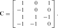
It is easy to verify that for these contrasts the assumption of symmetry holds rather more strongly, since the p values corresponding to the skewness are relatively larger. Specifically for these contrasts
and the respective p values for skewness and kurtosis tests are 0.8559 and 0.4862. As Rao (1948) points out, this symmetry is not surprising since these are linear combinations, and the contrasts are likely to fit the multivariate normality better than the original data. Since one can easily modify Program 1.1 or Program 1.2 to perform the above analysis on the contrasts z1, z2, and z3, we have not provided the corresponding SAS code or the output.
Mudholkar, McDermott and Srivastava (1992) suggest another simple test of multivariate normality. The idea is based on the facts that (i) the cube root of a chi-square random variable can be approximated by a normal random variable and (ii) the sample mean vector and the sample variance covariance matrix are independent if and only if the underlying distribution is multivariate normal. Lin and Mudholkar (1980) had earlier used these ideas to obtain a test for the univariate normality.
To test multivariate normality (of dimension say p) on the population with mean vector μ and a variance covariance matrix Σ, let y1,...,yn be a random sample of size n then the unbiased estimators of μ and Σ are respectively given by ![]() and S. Corresponding to ith observation we define,
and S. Corresponding to ith observation we define,

and
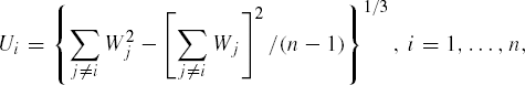
where
Let r be the sample correlation coefficient between (Wi,Ui), i = 1,...,n. Under the null hypothesis of multivariate normality of the data, the quantity, Zp = tanh−1(r) = ½ln![]() is approximately normal with mean μn,p = E(Zp) =
is approximately normal with mean μn,p = E(Zp) = ![]() , where A1(p) =
, where A1(p) = ![]() −.52p and A2(p) = 0.8p2 and variance, σn,p2 = var (Zp) =
−.52p and A2(p) = 0.8p2 and variance, σn,p2 = var (Zp) = ![]() , where B1(p) = 3 -
, where B1(p) = 3 - ![]() and B2(p) = 1.8p -
and B2(p) = 1.8p - ![]() . Thus, the test based on Zp to test the null hypothesis of multivariate normality rejects it at α level of significance if
. Thus, the test based on Zp to test the null hypothesis of multivariate normality rejects it at α level of significance if ![]() , where
, where ![]() is the right
is the right ![]() cutoff point from the standard normal distribution.
cutoff point from the standard normal distribution.
EXAMPLE 1
Testing Multivariate Normality, Cork Data (continued) In Program 1.3, we reconsider the cork data of C. R. Rao (1948) and test the hypothesis of the multivariate normality of the tree population.
/* Program 1.3 */
options ls=64 ps=45 nodate nonumber;
title1 'Output 1.3';
title2 'Testing Multivariate Normality (Cube Root Transoformation)';

data D1;
infile 'cork.dat';
input t1 t2 t3 t4 ;
/*
t1=north, t2=east, t3=south, t4=west
n is the number of observations
p is the number of variables
*/
data D2(keep=t1 t2 t3 t4 n p);
set D1;
n=28;
p=4;
run;
data D3(keep=n p);
set D2;
if _n_ > 1 then delete;
run;
proc princomp data=D2 cov std out=D4 noprint;
var t1-t4;
data D5(keep=n1 dsq n p);
set D4;
n1=_n_;
dsq=uss(of prin1-prin4);
run;
data D6(keep=dsq1 n1 );
set  D5;
dsq1=dsq**((1.0/3.0)-(0.11/p));
run;

proc iml;
use D3;
read all var {n p};
u=j(n,1,1);
use D6;
do k=1 to n;
setin D6 point 0;
sum1=0;
sum2=0;
do data;
read next var{dsq1 n1} ;
if n1 = k then dsq1=0;
sum1=sum1+dsq1**2;
sum2=sum2+dsq1;
end;
u[k]=(sum1-((sum2**2)/(n - 1)))**(1.0/3);
end;
varnames={y};
create tyy from u (|colname=varnames|);
append from u;
close tyy;
run;
quit;
data D7;
set D6; set tyy;
run;
proc corr data=D7 noprint outp=D8;
var dsq1;
with y;
run;
data D9;
set D8;
if _TYPE_ ^='CORR' then delete;
run;
data D10(keep=zp r tnp pvalue);
set D9(rename=(dsq1=r));
set D3;
zp=0.5*log((1+r)/(1-r));
b1p=3-1.67/p+0.52/(p**2);
a1p=-1.0/p-0.52*p;
a2p=0.8*p**2;
mnp=(a1p/n)-(a2p/(n**2));
b2p=1.8*p-9.75/(p**2);
ssq1=b1p/n-b2p/(n**2);
snp=ssq1**0.5;
tnp=abs(abs(zp-mnp)/snp);
pvalue=2*(1-probnorm(tnp));
run;
proc print data=D10;
run;The SAS Program 1.3 (adopted from Apprey and Naik (1998)) computes the quantities, Zp, μn,p, and σn.p using the expressions listed above. Using these, the test statistic |zn,p| and corresponding p value are computed. A run of the program results in a p value of 0.2216. We thus accept the hypothesis of multivariate normality. This conclusion is consistent with our earlier conclusion using the Mardia's tests for the same data set. Output corresponding to Program 1.3 is suppressed in order to save space.