6.4. Statistical Tests for Covariance Structures

In Chapter 5, we encountered the spherical or compound symmetric covariance structures as a required prerequisite for the univariate analysis of variance methods to be valid for the repeated measures data. It was suggested that one should first test if such a covariance structure can be assumed using the likelihood ratio tests. In many real world applications the hypothesis of spherical or compound symmetric covariance structure will be rejected. While the univariate analysis of variance approach is then invalidated, one may still pursue the (univariate-like) analysis using the asymptotic results based on the maximum likelihood theory. However, in such problems, first one should also determine the appropriate covariance structure so as to enable one to estimate the unknown parameters, including the ones represented in the covariance structure. As earlier, the likelihood ratio tests can be used to test such hypotheses. However, unlike the cases discussed in Chapter 5, it may not be possible to obtain a closed form test statistic when testing for the particular covariance structure. Fortunately, in the data analysis problems, such an issue is only secondary as long as the evaluation of the test statistics is computationally feasible and its theoretical properties are known.

Let y_p×1 be a p−variate normally distributed random vector with mean μ and the variance covariance matrix Σ. Suppose we have our data as a random sample y₁,...,yn from this population. The appropriate likelihood ratio test statistic for the null hypothesis,

H₀ : Σ has a given covariance structure

is given by,

where g(Σ|data) is same as the f(y₁,...,yn), the joint density function of y₁,...,yn and for optimization purposes, it is treated as a function of Σ for given data. Of course, any other unknown parameters, that may appear in the function g(.|data) will be replaced by their maximum likelihood estimates.

It may be noted that in certain problems and for the calculation of the denominator of L, the matrix Σ may not be completely unrestricted and from the very context of the problem at hand, it may still have some covariance structure. The likelihood ratio test can still be performed so long as this restricted parameter space itself contains as a subset, the parameter space restricted by H₀. A simple example of such a situation is when we want to test if a variance covariance matrix additionally has a compound symmetric structure while it is a priori assumed that this matrix already has a circular covariance structure — a structure which contains all compound symmetric variance covariance matrices as a further specialization. In Example 3, we consider yet another context where such a situation arises.

From the likelihood theory it follows that for large n, and under the null hypothesis, −2lnL approximately follows a chi-square distribution with f degrees of freedom, where the quantity f is computed as

f = number of unknown parameters in unstructured Σ− number of unknown parameters in Σ under the covariance structure specified by H₀.

For a better approximation, often a correction factor b known as the Bartlett's correction is multiplied to −2lnL and hence −2blnL is used as the modified test statistic. However, we will not concern ourselves with this modification in this chapter.

Often, instead of maximizing the likelihood, only a part of the likelihood which is invariant of the fixed effects is maximized. This results in what is known as the restricted maximum likelihood (REML) estimate of the variance covariance matrix. Using these estimates, another test statistic L^R instead of L defined above can be devised. Corresponding to L^R, the quantity −2lnL^R also follows a chi-square distribution and in fact, it is asymptotically equivalent to the test based on −2lnL. Since in PROC MIXED the default estimation is REML, the quantities reported under the default correspond to −2lnL^R rather than −2lnL.

Using SAS, a number of covariance structure choices can be adopted and hence tests for these can be performed using the MIXED procedure. Here we give a list of a few selected covariance structures. The complete list can be found in SAS/STAT Software: Changes and Enhancements through Release 6.12. Corresponding SAS options to be used in the REPEATED statement in PROC MIXED are indicated within the parentheses.

Linear Structures

In addition, one can test the null hypothesis (as well as perform the estimation) for any variance covariance matrix Σ, which can be represented as a linear combination of known matrices. Such a structure is called a linear covariance structure and is given by

where A₁,...,A_k are known matrices but the scalars c₁,...,c_k are all unknown and are functionally unrelated to each other. For example, the matrix

does have the above structure but the matrix

does not because the three parameters c₁ = σ², c₂ = σ²ρ and C₃ = σ²ρ² are essentially dependent on only two quantities namely, σ² and ρ and therefore are functionally related. The SAS option for linear structure is TYPE =LIN(k) which is specified as part of the REPEATED statement.

It may be remembered that presently we are dealing with the fixed effects models of the type y_i = μ+ϵ_i only and hence the variance covariance matrix of y_i is the same as the variance covariance matrix of ϵ_i. If the p by 1 vector μ corresponds to fewer than p parameters and is linearly expressed as μ = Xβ for some design matrix X then the MODEL statement can be used to specify such details for fixed effects. In the REPEATED statement of the MIXED procedure, one can specify the covariance structure of ϵ_i and hence in the present case, for y_i. This will not be the case if the model also has some other random effects.

From the expression of L, it is clear that,

where and are the maximum likelihood estimators of Σ under H₀ and without any restrictions on Σ, respectively. The two terms in the above expression can be obtained by executing the MIXED procedure twice, for the appropriate models and under appropriate covariance structures, which are specified as the TYPE = option in the REPEATED statements. The option TYPE =UN will result in the value of . The appropriate option to obtain depends on what H₀ is.

EXAMPLE 1

Testing Covariance Structure, Glucose Data Six volunteers were observed for the blood glucose levels over a period of time after eating a certain test meal. Measurements were taken 15 minutes before the meal, immediately before (0 hours) and then at every half an hour for the next two hours. Later, hourly readings were taken for the next four hours. The measurements from time point 0 onward are denoted by y₁,...,y₉. The time points are represented by the variable TIMEPT in the program. The experiment was repeated six times with the meals taken at different times of the day, thus giving the six treatments (represented by GROUP in the program). Any carryover effect of treatments was assumed to be nonexistent. Data were obtained from Crowder and Hand (1990, p. 14); we have replaced the two missing values in the data set by certain estimates.

To do any meaningful analysis, we must first determine the appropriate covariance structure for the errors. To begin with, an AR(1) structure seems a potential choice but the observations are not made at equal time intervals. In view of this, a Markov covariance structure given by Σ = (σ_ij), σ_ij = σ²ρ^d_ij, where d_ij = |t_i − t_j| is the time elapsed between i^th and j^th repeated measures, can be used. We will therefore test the null hypothesis that the error covariance structure is of the Markov type. As there are no other random effects (except of course subjects on which repeated measures are taken) in the present context, the test on the covariance structure for error is the same as that for the dependent variable. Consequently, we will test for the Markov covariance structure after correcting for the fixed effects present in the model, namely, the GROUP, TIMEPT and their interaction. In SAS, the Markov structure is referred to as the Spatial power structure and is specified by the option TYPE = SP(POW) (V_BLE) where V_BLE defines the variable taking values as time points t₁,..., t_p.

A SAS program for this test is presented in Program 6.1. First of all, the data on y₁,..., y₉ at the nine time points should be arranged on a single variable y, at various levels of the variable TIMEPT. This is done using the first part of the code presented in Program 6.1. Output 6.1 follows.

/* Program 6.1 */

options ls =64 ps=45 nodate nonumber;
title1 'Output 6.1';
title2 'Test for Markov Covariance Structure: Glucose Data';
data a;
infile 'glucose.dat' obs=36;
input id group$ before y1-y9;
run;
data c;
set a;
array t{9} y1-y9;
subj+1;
do timept=1 to 9;
y=t{timept};
if timept = 1 then realtime = 0;
if timept = 2 then realtime = .5;
if timept = 3 then realtime = 1;
if timept = 4 then realtime = 1.5;
if timept = 5 then realtime = 2;
if timept = 6 then realtime = 3;
if timept = 7 then realtime = 4;
if timept = 8 then realtime = 5;
if timept = 9 then realtime = 6;
output;
end;
drop y1-y9;
run;
proc mixed method=ml;
class subj  group timept;
model y= group timept group*timept;
repeated/type=un subject=subj;
title3 'Unstructured Covariance';
run;
proc mixed method=ml;
class subj group timept;
model y=group timept group*timept;
repeated/type=sp(pow)(realtime) subject=subj;
title3 'Markov Covariance';
run;

Example 6.1. Output 6.1

Test for Markov Covariance Structure: Glucose Data
                      The MIXED Procedure

                    Unstructured Covariance
                Model Fitting Information for Y

            Description                        Value

            Observations                    324.0000
            Log Likelihood                  -288.269
            Akaike's Information Criterion  -333.269

Schwarz's Bayesian Criterion    −418.336
            -2 Log Likelihood               576.5388
            Null Model LRT Chi-Square       211.7630
            Null Model LRT DF                44.0000
            Null Model LRT P-Value            0.0000


                       Markov Covariance
                Model Fitting Information for Y

            Description                        Value

            Observations                    324.0000
            Log Likelihood                  -385.092
            Akaike's Information Criterion  -387.092
            Schwarz's Bayesian Criterion    -390.873
            -2 Log Likelihood               770.1850
            Null Model LRT Chi-Square        18.1168
            Null Model LRT DF                 1.0000
            Null Model LRT P-Value            0.0000

Note that the variable REALTIME which is different from the variable TIMEPT, takes values corresponding to the actual time elapsed. This information is needed in specifying the covariance structure.

To compute the likelihood ratio L, the two likelihood functions are to be maximized separately. This is done using the option METHOD = ML in the PROC MIXED statement in the corresponding two executions. As explained earlier, the corresponding fixed effects are to be specified in the MODEL statement. The options TYPE = UN and TYPE = SP(POW)(REALTIME) are used for specifying the appropriate covariance structures used in the calculations of the denominator and the numerator of L. The results of these two runs of PROC MIXED are reported in Output 6.1.

Since

rather than working with the individual maximized likelihoods, it suffices to only know −2 times their natural logarithm. Fortunately, these are reported as −2 Log Likelihood in the output. Thus the observed value of the chi-square test statistic is χ² = −2lnL = 770.1850−576.5388 = 193.6462. This test statistic follows a chi-square distribution with degrees of freedom f = Null Model LRT df (Under H₀) − Null Model LRT df (Unrestricted) = 44 − 1 = 43.

This observed value of the test statistics is highly significant at any reasonable level of significance (such as 5% or 1%) and hence the null hypothesis of Markov covariance structure can be rejected.

Testing for Linear Structures As discussed earlier, a variance covariance matrix Σ is said to have a linear structure if it can be written as, Σ = c₁A₁+...+c_kA_k, for some k and for some known matrices A₁,..., A_k. The parameters c₁,...,c_k are unknown and assumed to be functionally not related to each other, or can be reparametrized to do so.

There are a number of models and consequently a number of situations, where the variance covariance matrix has a linear structure. The hypothesis about such covariance structures can also be tested using the MIXED procedure. For this the option TYPE = LIN(k), where k is the number of parameters in the linear structure can be used in the REPEATED statement. However, the known matrices A_i corresponding to parameters c_i, i = 1,...,kare to be specified separately in a data set. We will illustrate this using the cork data discussed extensively in the earlier chapters.

EXAMPLE 2

Cork Data, Testing Circular Structure for Measurements on a Tree We have already provided PROC IML code to test the circulant covariance structure in Chapter 5. The approach here provides an alternative (although not universally applicable due to convergence problems) approach. Due to the very nature of cork data, where the measurements on the trees were taken along four directions namely, North, East, South and West, the assumption of circular covariance structure seems to be a viable one. The variance covariance matrix,

can be written either as

or as

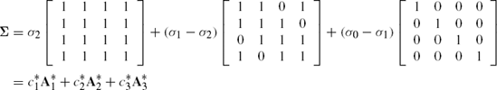
among certain other choices. We will however use the first representation. Clearly, k = 3 and A₁, A₂ and A₃ are known. The fact that these matrices are to be retrieved from another data set titled CIRC has been specified in the option LDATA = CIRC in the REPEATED statement. The PARMS statement is optional within the code but has been used to provide some initial guesses of the parameters σ₀, σ₁ and σ₂ for the iterative process. Such a specification is helpful and highly recommended to attain the convergence because often during the iterations the parameters may be estimated by quantities which may violate the required positive definiteness of the matrix Σ, thereby making the likelihood function unbounded and growing indefinitely. It may be pointed out that for the present example, the convergence is not obtained unless the PARMS statement with appropriate initial values is added.

Returning to the specification of matrices A₁, A₂ and A₃, these are specified row by row in the data set CIRC. The variable PARM taking values 1, 2 and 3, specifies which parameter — first, second or third, that is, c₁, c₂ or C₃ — does the particular matrix correspond to. Accordingly, in the output, these parameters are referred to as LIN(1), LIN(2) and LIN(3) respectively.

The program for this testing problem is shown in Program 6.2. The corresponding output appears in Output 6.2. The chi-square test statistic χ² = −2lnL= 811.1686 −791.4164 = 19.7522 at degrees of freedom 9 − 2 = 7 is significant at any reasonable level of significance. We therefore reject the hypothesis of circulant structure.

/* Program 6.2 */

options ls =64 ps=45 nodate nonumber;
title1 'Output 6.2';

title2 'Test for Linear Structure: Circulant for Cork Data';
data cork;
infile 'cork.dat';
input n e w s;
data cork1;
set cork;
array t{4} n e s w;
tree+1;
do dir = 1 to 4;
dir1 = dir;
y = t{dir};
output;
end;
drop n e s w;
run;
data circ;
input parm row col1-col4;
datalines;
1 1 1 0 0 0
1 2 0 1 0 0
1 3 0 0 1 0
1 4 0 0 0 1
2 1 0 1 0 1
2 2 1 0 1 0
2 3 0 1 0 1
2 4 1 0 1 0
3 1 0 0 1 0
3 2 0 0 0 1
3 3 1 0 0 0
3 4 0 1 0 0
;
proc mixed data =cork1 method = ml;
class tree dir;
model y =dir;
repeated/ type =un subject = tree;
title3 'Unstructured Covariance';
run;
proc mixed data = cork1 method = ml;
class tree dir;
model y = dir;
repeated/type = lin(3) ldata = circ subject = tree;
parms (190) (30) (70);
title3 'Circulant';
run;

Example 6.2. Output 6.2

Test for Linear Structure: Circulant for Cork Data
                      The MIXED Procedure

                    Unstructured Covariance
                Model Fitting Information for Y

            Description                        Value

            Observations                    112.0000
            Log Likelihood                  -395.708
            Akaike's Information Criterion  −405.708
            Schwarz's Bayesian Criterion    −419.301
            -2 Log Likelihood               791.4164

Null Model LRT Chi-Square       150.0319
            Null Model LRT DF                 9.0000
            Null Model LRT P-Value            0.0000


                           Circulant
                Model Fitting Information for Y

            Description                        Value

            Observations                    112.0000
            Log Likelihood                  −405.584
            Akaike's Information Criterion  −408.584
            Schwarz's Bayesian Criterion    −412.662
            -2 Log Likelihood               811.1686
            PARMS Model LRT Chi-Square       78.0542
            PARMS Model LRT DF                2.0000
            PARMS Model LRT P-Value           0.0000

We have already emphasized the usefulness of specifying the initial guess(es) of the parameters in the PARMS statement. In fact, in our experience, we have encountered many data sets where despite our best efforts by specifying the good initial guesses, we could not succeed in obtaining the convergence. Fortunately, in the case of circulant covariance structure, we do have an alternative namely, that given in Program 5.4.

Prespecified Known Variance Covariance Matrix In many situations, it is often of interest to test the hypothesis that the population variance covariance matrix is equal to a given known positive definite matrix. This can be done using a combination of TYPE = LIN(k) and NOITER options along with PARMS statement. The following example illustrates the approach.

EXAMPLE 3

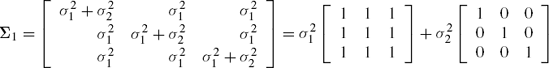
Quality Control for Car Door Panels, Warpage Data During the manufacturing process in the automotive industry, an undesirable amount of warpage on car door panels is often observed. During a manufacturing process, warpage measurements are taken at three different locations on the same car door panel. The three observations can be treated as repeated measures. The two sources of variation during the process are the variations within and between the car door panels denoted respectively as σ₁² and σ₂². Thus the variance covariance matrix of three measurement on the same panel will have a compound symmetric structure given by,

For control chart purposes, it is believed that σ₁²= 1.0 and σ₂²=0.1. Thus Σ = Σ₀=11′+(0.1)I is a known compound symmetric matrix. Periodically, checks are to be made to see if the process is stable and that the variability of the process has not changed. Thus, it is appropriate to test the hypothesis

Data on fifteen panels were collected for all three measurements and are reported as part of Program 6.3. Clearly, k=2. Thus, we use the option TYPE = LIN(2) in the REPEATED statement. As in the previous example, the matrices A₁=11′ and A₂=I are specified in the data set MATRIX. We use the PARMS statement with initial guesses for c₁ and C₂ as 0.1 and 1.0 respectively but allow no iterations for maximum likelihood estimation using the option NOITER. Consequently, no iterations will take place and the matrix Σ will remain as Σ₀ = c₁A₁ +c₂A₂ with c₁ = 0.1 and C₂ = 1.0 for the computation of likelihood.

However, in this particular context, we may also note that regardless of any shifts in the process variances, the compound symmetric structure of Σ will still be intact. Thus, to maximize the denominator of L, one should still use the compound symmetric structure Σ=c₁A₁+c₂A₂, with c₁ and C₂ unknown. Therefore, we must use the TYPE =CS option rather than TYPE =UN in this case as has been done in Program 6.3. Output 6.3 follows.

/* Program 6.3 */

options ls =64 ps=45 nodate nonumber;
title1 'Output 6.3';
title2 'Test for Sigma =Sigma_0: Warpage Data';
data warpage;
input y1 y2 y3;
lines;
3.3 3.7 3.8
4.1 4.3 4.9
2.1 1.9 2.0
1.8 1.4 2.2
3.9 3.9 3.7
2.5 2.7 2.5
4.4 3.9 4.0
3.3 3.7 4.0
4.4 3.8 4.2
1.1 1.7 1.5
1.8 1.4 1.8
4.4 4.8 4.3
3.4 3.4 3.9
2.9 2.5 2.4
3.6 3.1 3.8
;
data warpage1;
set warpage;
array t{3} y1-y3;
panel+1;
do location = 1  to 3;
y = t{location};
output;
end;
drop y1-y3;
run;
data matrix;
input parm row col1-col3;
datalines;
1 1 1 1 1
1 2 1 1 1
1 3 1 1 1
2 1 1 0 0
2 2 0 1 0
2 3 0 0 1
;
proc mixed data =warpage1 method = ml;
class panel location ;
model y =location ;
repeated/ type =cs subject = panel;
title3 'Compound Symmetry';

run;
proc mixed data =warpage1 method = ml;
class panel location ;
model y =location ;
parms (1) (.1)/noiter;
repeated/ type =lin(2) ldata =matrix subject = panel;
title3 'Known Fixed Sigma_0';
run;

Example 6.3. Output 6.3

Test for Sigma =Sigma_0: Warpage Data
                      The MIXED Procedure

                       Compound Symmetry
                Model Fitting Information for Y

            Description                        Value

            Observations                     45.0000
            Log Likelihood                  -32.9845
            Akaike's Information Criterion  -34.9845
            Schwarz's Bayesian Criterion    -36.7911
            -2 Log Likelihood                65.9690
            Null Model LRT Chi-Square        65.2826
            Null Model LRT DF                 1.0000


                      Known Fixed Sigma_0
                Model Fitting Information for Y

            Description                        Value

            Observations                     45.0000
            Log Likelihood                  -33.6813
            Akaike's Information Criterion  -35.6813
            Schwarz's Bayesian Criterion    -37.4880
            -2 Log Likelihood                67.3627
               Test for Sigma =Sigma_0: Warpage Data

From Output 6.3, it is evident that −2lnL= 67.3627 − 65.9690 = 1.3937. This follows a chi-square distribution with degrees of freedom equal to the difference between the Null Model LRT DF under two scenarios. Since no parameters have been estimated when Σ has been specified as Σ₀, the degrees of freedom for our χ² test statistics obtained from the likelihood ratio is 1. Since the observed value of 1.3937 is quite small and smaller than the χ² cut off point at any reasonable level of significance, we do not reject the null hypothesis in this case and claim that the two components of the process variability are unchanged.

Finally a few comments on choosing a covariance structure among several competing ones are in order. It is possible that for two different covariance structures, when LR tests are applied, they deem both covariance structures as acceptable. Which of the two should one choose? While no conclusive well defined preference policy can be laid out, certain measures can still be used to evaluate such preferences. These are Akaike's and Schwartz's information criteria defined earlier and popularly referred to as AIC and BIC respectively. The larger value of these criteria indicates a higher degree of preference. It may however be remarked that recent simulation studies by Keselman, Algina, Kowalchuk and Wolfinger (1998) indicate that both of these methods often fail to identify the true covariance structure, although AIC performs a little better than BIC in this respect.

Assuming no random effects, the tests presented above require that the fixed effect part of the model remain the same while maximizing the two likelihoods. However, estimating the appropriate fixed effect part of the model is itself a step in modeling and thus the fixed effects will seldom be known a priori. Diggle, Liang and Zeger (1995) suggest that to determine the appropriate covariance structure, one may use the saturated model. Once an appropriate covariance structure has been determined, the modeling of fixed effects and its reduction to a more parsimoneous model can be done under the selected covariance structure.

As an ad-hoc procedure, the above two stage procedure can also be applied when the model contains some random effects as well. In this case, for the selection of an appropriate covariance structure, residuals instead of data on response variables should be used. These residuals may be obtained by initially fitting the saturated fixed and random effect parts of the model under the spherical covariance structure. Once these are obtained, two separate runs (under H₀ and unrestricted respectively) of MIXED procedure as detailed earlier will enable one to test the hypothesis on the error covariance structure.