
3.10. Regression Diagnostics
As in univariate regression, to assess various assumptions on the multivariate regression model and the validity of the model, diagnostics should be an integral part of the analysis. Such diagnostics tools also include data scrutiny to notice any striking or unusual features present in the data. Certain quantities such as the matrices of predicted values, Ŷ=XB=X(X′X)−1X′Y = PY, of residuals, ![]() =Y−Ŷ=(I−P)Y, and of estimated error variances and covariances,
=Y−Ŷ=(I−P)Y, and of estimated error variances and covariances, ![]() =E/(n−k−1)=Y′(I−P)Y/(n−k−1), where P=X(X′X)−1X′=(pij) is the projection matrix also known as the hat matrix, play a key role in such analyses. We will present certain aspects of these analyses in this section.
=E/(n−k−1)=Y′(I−P)Y/(n−k−1), where P=X(X′X)−1X′=(pij) is the projection matrix also known as the hat matrix, play a key role in such analyses. We will present certain aspects of these analyses in this section.
3.10.1. Assessing the Multivariate Normality of Error
One of the basic assumptions needed to perform the statistical tests under Equation 3.2 is that the rows of ɛ are independent and the multivariate normally distributed. This assumption can be checked graphically using a Q−Q plot or analytically by applying formal statistical tests, as presented in Chapter 1, on the residuals.
Let ![]() be the rows of ɛ and
be the rows of ɛ and ![]() be that of
be that of ![]() . If the multivariate normality assumption holds, the squared distances d2i
. If the multivariate normality assumption holds, the squared distances d2i![]() , i = 1,...,n will be distributed approximately as chi-squares each with p degrees of freedom. Although these are not theoretically independent, for a model well fit the correlations will be weak. Hence a Q-Q plot of di2 against the χp2 quantiles will indicate a multivariate normality assumption being acceptable if the points on the plot fall around a 45° angle line passing through the origin. Formal tests were used in Chapter 1 for testing the multivariate normality of data. The same tests can be adopted in the present context after some modifications for the residual vectors
, i = 1,...,n will be distributed approximately as chi-squares each with p degrees of freedom. Although these are not theoretically independent, for a model well fit the correlations will be weak. Hence a Q-Q plot of di2 against the χp2 quantiles will indicate a multivariate normality assumption being acceptable if the points on the plot fall around a 45° angle line passing through the origin. Formal tests were used in Chapter 1 for testing the multivariate normality of data. The same tests can be adopted in the present context after some modifications for the residual vectors ![]() .
.
EXAMPLE 8
Multivariate Normality Test We use the data of Dr. William D. Rohwer reported in Timm (1975, p. 281, 345). Interest is in predicting the performance of a school child on three standardized tests, namely, Peabody Picture Vocabulary Test (y1), Raven Progressive Matrices Test (y2), and Student Achievement Test (y3) given the sums of the numbers of correct items out of 20 (on two exposures) to five types of paired-associated (PA) tasks. The five PA tasks are: named (x1), still (x2), named still (x3), named action (x4), and sentence still (x5). The data correspond to 32 randomly selected school children in an upper-class, white residential school.
We fit the multivariate linear regression model with three responses y1, y2, y3 and five independent variables x1, ..., x5 as
Y32×3=X32×6B6×3+ɛ32×3,
In the SAS Program 3.9, the OUTPUT statement
output out = b, r=e1 e2 e3 p=yh1 yh2 yh3 h=p_ii;
is used to store the residuals (option R = E1 E2 E3), predicted values (option P = YH1 YH2 YH3), and the diagonal elements of the hat matrix (option H=P_II) in a SAS data set named B using the option OUT=B. The residuals are then used to calculate di2. Selected parts of the output are shown in Ouput 3.9.
/* Program 3.9 */
options ls=64 ps=45 nodate nonumber;
    title1 'Output 3.9';
    title2 'Multivariate Regression Diagnostics';
    data rohwer;
    infile 'rohwer.dat' firstobs=3;
    input ind y1 y2 y3 x1−x5;
    run;

    /* Store all the residuals, predicted values and the diagonal
    elements (p_ii) of the projection matrix, (X(X'X)^−1X'), in a
    SAS data set (we call it B in the following) */
    proc reg data=rohwer;
    model y1−y3=x1−x5/noprint;
    output out=b r=e1 e2 e3 p=yh1 yh2 yh3 h=p_ii;

    /* Test for multivariate normality using the skewness and kurtosis
    measures of the residuals.  Since the sample means of the residuals
    are zeros, Program 1.2 essentially works. */
    proc iml;
    use b;
    read all var {e1 e2 e3} into y;
    n = nrow(y) ;
    p = ncol(y) ;
    dfchi = p*(p + 1)*(p+2)/6;
    q = i(n) − (1/n)*j(n,n,1);
    s = (1/(n))*y`*q*y; /* Use the ML estimate of Sigma */
    s_inv = inv(s);
    g_matrix = q*y*s_inv*y`*q;
    beta1hat = ( sum(g_matrix#g_matrix#g_matrix) )/(n*n);
    beta2hat =trace( g_matrix#g_matrix )/n;
    kappa1 = n*beta1hat/6;
    kappa2 = (beta2hat − p*(p+2) ) /sqrt(8*p*(p+2)/n);
    pvalskew = 1 − probchi(kappa1,dfchi);
    pvalkurt = 2*( 1 − probnorm(abs(kappa2)) ) ;
    print beta1hat ;
    print kappa1 ;
    print pvalskew;
    print beta2hat ;
    print kappa2 ;
    print pvalkurt;

    /* Q-Q plot for checking the multivariate normality using
    Mahalanobis distance of the residuals;*/
    data b;
    set b;
    totn=32.0;  /* totn is the number of observations */
    k=5.0;  /* k is the no. of indep. variables */
    p=3.0; /* p is the number of dep. variables */
    proc princomp data=b cov std out=c noprint;
    var e1−e3;
    data sqd;
    set c;
    student=n_;
    dsq=uss(of prin1−prin3);
    dsq=dsq*(totn-k−1)/(totn−1);
    * Divide the distances by (1−p_ii);
    dsq=dsq/(1−p_ii);
data qqp;
set sqd;
proc sort;
by dsq;
data qqp;
set qqp;
stdnt_rs=student;
chisq=cinv(((n_-.5)/ totn),p);
proc print data=qqp;
var stdnt_rs dsq chisq;
* goptions for the gplot;
filename gsasfile "prog39a.graph";
goptions reset=all gaccess=gsasfile autofeed dev=pslmono;
goptions horigin=1in vorigin=2in;
goptions hsize=6in vsize=8in;
title1 h=1.5 'Q-Q Plot for Assessing Normality';
title2 j=l 'Output 3.9';
title3 'Multivariate Regression Diagnostics';
proc gplot data=qqp;
plot dsq*chisq='star';
label dsq = 'Mahalanobis D Square'
chisq= 'Chi-Square Quantile';
run;
* Q-Q plot for detection of outliers using Robust distance;
* (Section 3.10.3);
data qqprd;
set sqd;
rdsq=((totn-k-2)*dsq/(totn-k−1))/(1−(dsq/(totn-k−1)));
proc sort;
by rdsq;
data qqprd;
set qqprd;
stdnt_rd=student;
chisq=cinv(((n_-.5)/ totn),p);
proc print data=qqprd;
var stdnt_rd rdsq chisq;
filename gsasfile "prog39b.graph";
title1 h=1.5 'Q-Q Plot of Robust Squared Distances';
title2 j=l 'Output 3.9';
title3 'Multivariate Regression Diagnostics';
proc gplot;
plot rdsq*chisq='star';
label rdsq = 'Robust Mahalanobis D Square'
chisq= 'Chi-Square Quantile';
run;
* Influence Measures for Multivariate Regression;
* (Section 3.10.4);
* Diagonal Elements of Hat (or Projection) Matrix;
data hat;
set sqd;
proc sort;
by p_ii;
data hat;
set hat;
stdnt_h=student;keep stdnt_h p_ii;
run;
* Cook's type of distance for detection of influential obs.;
data cookd;
set sqd;
csq=dsq*p_ii/((1−p_ii)*(k+1));
proc sort;
by csq;
data cookd;
set cookd;
stdnt_co=student;
keep stdnt_co csq;
run;
* Welsch-Kuh type statistic for detection of influential obs.;
data wks;
set qqprd;
wksq=rdsq*p_ii/(1−p_ii);
proc sort;
by wksq;
data wks;
set wks;
stdnt_wk=student;
keep stdnt_wk wksq;
run;
* Covariance Ratio for detection of influential obs.;
data cvr;
set qqprd;
covr=((totn-k-2)/(totn-k-2+rdsq))**(k+1)/(1−p_ii)**p;
covr=covr*((totn-k−1)/(totn-k-2))**((k+1)*p);
proc sort;
by covr;
data cvr;
set cvr;
stdnt_cv=student;
keep stdnt_cv covr;
run;
* Display of Influence Measures;
data display;
merge hat cookd wks cvr;
title2 'Multivariate Regression Diagnostics';
title3 'Influence Measures';
proc print data=display noobs;
var stdnt_h p_ii stdnt_co csq stdnt_wk wksq stdnt_cv covr;
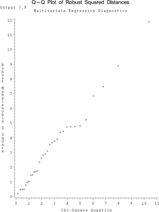
run;The Q−Q plot of ordered di2 (denoted by DSQ in Program 3.9) against the quantiles of χ32 (denoted by CHISQ) presented in Output 3.9 seems to indicate no violation of multivariate normality assumption.
Using a modification of Program 1.2 (code provided in Program 3.9) Mardia's skewness and kurtosis tests (see Chapter 1) are performed on the residuals. The p value for the test based on skewness (denoted by PVALSKEW in Program 3.9) is 0.8044 and that for the test based on kurtosis (denoted by PVALKURT) is 0.4192. The corresponding output has been eliminated. In view of these large p values, we see no evidence of any violation of multivariate normality assumption. One can also perform the test due to Mudholkar, McDermott, and Srivastava (1992). For the present dataset, the conclusion obtained is the same.

3.10.2. Assessing Dispersion Homogeneity
One of the important components of residual analysis in univariate regression is the residual plots. A plot of (studentized) residual values drawn against the predicted values may indicate various possible violations of the assumptions of the regression model. For example, a plot which funnels out (or funnels in) is considered to be an indication of heterogeneity of error variance, in that the error variance may depend on certain functions of the predicted values or the independent variables.
For multivariate regression, a similar residual plot may be suggested based on the following motivation. Suppose in the univariate situation the absolute values of the (studentized) residuals (instead of the residuals) are plotted against the absolute values of the corresponding predicted values. Then various shapes and features in this plot can be utilized to determine the violations of different aspects of the assumptions in the model. Since in this plot the absolute values of the studentized residuals are being used, a plot in the original residuals which was funneling out, for example, will now have only the upper half of the funnel in this plot. This fact can be utilized to suggest a residual plot in (diϵ, diy), i = 1,...,n, where

and where Ŷi′ is the ith row of Ŷ, i = 1,...,n. We note that the quantities diϵ and diy respectively are the Mahalanobis distances of the vectors ϵi and Ŷi from the origin. We will call such a plot based on these two distances a D-D plot.
EXAMPLE 9
D-D Plot, Air Pollution Data Daily measurements on independent variables, wind speed (x1) and amount of solar radiation (x2), and dependent variables indicating the amounts of CO(y1), NO(y2), NO2(y3), O3 (y4) and HC(y5) in the atmosphere were recorded at noon in the Los Angeles area on 42 different days. One of the problems is to predict the air-pollutants measured in terms of y1 through y5 given the two predictors x1 and x2. We fit a multivariate regression model by taking only y3 and y4 as dependent variables and x1 and x2 as the independent variables. The logarithmic transformation was applied on all four variables. The D-D plot to assess the homogeneity of dispersion is considered here. Thus, we plot (diϵ vs. diy), which are computed using the formulas given above. The data set as well as the SAS code are given in Program 3.10. The data are courtesy of G. C. Tiao. In the Program 3.10 the distances diy and diϵ are denoted respectively by DSQ1 and DSQ2. The corresponding D-D plot is presented in Output 3.10.
/* Program 3.10 */
options ls=64 ps=45 nodate nonumber;
    title1 'Output 3.10';
    title2 'Multivariate Regression: D-D Plot';
    * The data set containing independent and dependent variables.;
    data pollut;
    infile 'airpol.dat' firstobs=6;
    input x1 x2 y1−y5;
    * Make transformations if necessary;
    data pollut;
    set pollut;
    x1=log(x1);
x2=log(x2);
y1=log(y1);
y2=log(y2);
y3=log(y3);
y4=log(y4);
y5=log(y5);
proc reg data=pollut;
model y3 y4=x1 x2/noprint;
output out=b r=e1 e2 p=yh1 yh2 h=pii;
/* Univariate residual plots;
proc reg data=pollut;
model y3 y4=x1 x2 /noprint;
plot student.*p.;
title2 'Univariate Residual Plots';
run;
*/
* The Mahalanobis distances of residuals and predicted values;
proc iml;
use b;
read all var {e1 e2} into ehat;
read all var {yh1 yh2} into yhat;
read all var {pii} into h;
n = nrow(ehat);
p = ncol(ehat);
k = 2.0; *The no. of independent variables in the model;
sig=t(ehat)*ehat;
sig=sig/(n−k−1); /* Estimated Sigma */
dsqe=j(n,1,0);
dsqyh=j(n,1,0);
do i = 1 to n;
dsqe[i,1]=ehat[i,]*inv(sig)*t(ehat[i,])/(1−h[i]);
dsqyh[i,1]=yhat[i,]*inv(sig)*t(yhat[i,])/h[i];
end;
dsqe=sqrt(dsqe);
dsqyh=sqrt(dsqyh);
dsqpair=dsqyh||dsqe;
varnames={dsq1 dsq2};
create ndat1 from dsqpair (|colname=varnames|);
append from dsqpair;
close ndat1;
* D-D Plot;
data ndat1;
set ndat1;
filename gsasfile "prog310.graph";
goptions reset=all gaccess=gsasfile autofeed dev=pslmono;
goptions horigin=1in vorigin=2in;
goptions hsize=6in vsize=8in;
title1 h=1.5 'D-D Plot';
title2 j=l 'Output 3.10';
title3 'Residual Analysis: Multivariate Regression';
proc gplot data=ndat1;
plot dsq2*dsq1='star';
label dsq1='Distance of Predicted Value'
dsq2='Distance of Residual';
run;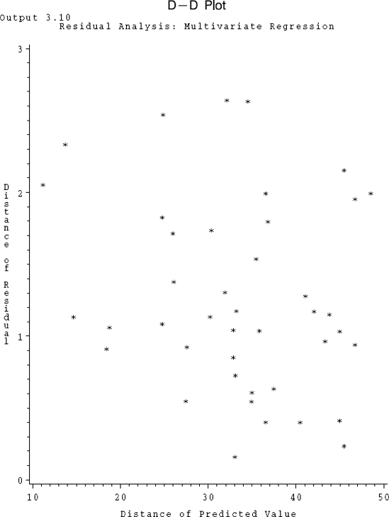
The plot clearly seems to show an increasing trend indicating that there may be some heterogeneity of error dispersion. A look at individual univariate studentized plots (not shown here) also supports this conclusion.
3.10.3. Outliers
Formal or graphical tests for multivariate normality may sometimes fail due to the presence of outliers in the data. Observations which are unusual in the sense that they violate certain model assumptions are outliers. A simple method of detection of outliers in a multivariate normal distribution case has been discussed in Chapter 2. It involves plotting robust Mahalanobis distances against the corresponding quantiles (Q-Q plot) of an appropriate chi-square distribution. This method can be applied on residuals to detect any outliers in multivariate regression analysis set up.
Analogous to the discussion in Chapter 2, we define
where ![]() /(n−k−2), and
/(n−k−2), and ![]() is the n − 1 by p residual matrix obtained by fitting the multivariate regression model Y=XB+
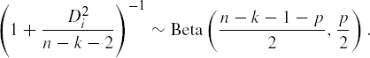
is the n − 1 by p residual matrix obtained by fitting the multivariate regression model Y=XB+![]() without the ith observation. As in Chapter 2, a relationship between the squared Mahalanobis distance di2 and its robust version, Di2 exists and is given by
without the ith observation. As in Chapter 2, a relationship between the squared Mahalanobis distance di2 and its robust version, Di2 exists and is given by
which is also a Hotelling T2 statistic. In the absence of any outliers the quantity
follows an Fp,n−k−1−p distribution. However, for large samples (such that n−k−1−p is large), the distribution of Di2 is approximately χp2 and this fact will be utilized to identify outliers in a Q-Q plot.
EXAMPLE 8
Detection of Outliers, Rohwer's Data (continued) SAS code given in Program 3.9 also computes di2 (DSQ) and Di2 (RDSQ) and then prints them in an increasing order of magnitude for this data set. The Di2 values along with the corresponding chi-square quantiles (CHISQ) are listed in Output 3.9 along with a Q-Q plot of these values. The largest Di2 is 11.87 corresponding to the 25th observation (listed under the variable STDNT_RD in the output). Since this is not very large compared to the corresponding χ32 quantile we conclude that there are no outliers in this data set. The corresponding Q-Q plot also supports this conclusion.
Example 3.9. Output 3.9
Multivariate Regression Diagnostics
              Q-Q Plot of Robust Squared Distances

             OBS    STDNT_RD      RDSQ      CHISQ

               1       15        0.1772     0.1559
               2       10        0.4521     0.3360
               3        6        0.4698     0.4864
               4        4        0.4809     0.6253
               5        2        0.7605     0.7585
               6       18        0.9489     0.8888
               7       22        1.0047     1.0181
               8       26        1.4352     1.1475
               9       16        1.4545     1.2780
              10       11        1.6509     1.4103
              11       28        1.6719     1.5452
              12       24        1.7299     1.6834
              13       13        2.3245     1.8256
              14       19        2.5938     1.9725
              15       20        2.7996     2.1250
              16        3        2.8882     2.2838
              17       30        3.0811     2.4501
              18        7        3.5062     2.6250
              19        1        3.6494     2.8099
              20       12        3.7542     3.0065
              21       27        3.8898     3.2169
              22        5        4.3593     3.4438
              23       23        4.4198     3.6906
              24        8        4.7224     3.9617
              25       17        4.7321     4.2636
              26       29        4.7502     4.6049
              27       32        4.7893     4.9989
              28        9        5.2072     5.4670
              29       21        6.8286     6.0464
              30       31        7.4628     6.8124
              31       14        8.8648     7.9586
32 25 11.8711 10.3762 |
If so desired, formal statistical tests to detect outliers in the context of multivariate regression can be used. One such test has been derived by Naik (1989). Instead of ![]() he utilized the uncorrelated best linear unbiased scalar (BLUS) residuals (Theil, 1971). The resulting test statistic is Mardia's kurtosis measure of BLUS residuals. We will not discuss this approach here. However, SAS code using PROC IML can easily be developed for this method.
he utilized the uncorrelated best linear unbiased scalar (BLUS) residuals (Theil, 1971). The resulting test statistic is Mardia's kurtosis measure of BLUS residuals. We will not discuss this approach here. However, SAS code using PROC IML can easily be developed for this method.
3.10.4. Influential Observations
Influential observations are those unusual observations which upon dropping from the analysis yield results which are drastically different from the results that were otherwise obtained. They are often contrasted from outliers by the fact that the presence of outliers in the data does not affect the results to the extent the influential observations do. One of the important developments in the recent univariate regression analysis literature has been the introduction of the concept of influential observations and statistical methods for detection of these observations. See Cook and Weisberg (1982). Here we discuss some of the approaches considered in Hossain and Naik (1989). It must be emphasized that these methods are not substitutes for one another and must be used in conjunction with each other.
The Hat Matrix Approach The projection or hat matrix is defined as P=X(X′X)−1X′. Let pii be the ith diagonal element of P. It is known that 0 ≤ pii ≤ 1 and tr
P=![]() . Hence the average of pii, i = 1,...,n, is
. Hence the average of pii, i = 1,...,n, is ![]() . Belsley, Kuh, and Welsch (1980) defined the observation i corresponding to which pii ≥
. Belsley, Kuh, and Welsch (1980) defined the observation i corresponding to which pii ≥ ![]() as a leverage point. A leverage point is a potential influential observation. The influence in this case is entirely due to one or more independent variables.
as a leverage point. A leverage point is a potential influential observation. The influence in this case is entirely due to one or more independent variables.
An observation may be influential entirely or in part due to one or more dependent variables. Such observations can be determined by using the residuals. For example, the distances di2 or the robust distances Di2 computed from the residuals can be used for this purpose. Thus an observation detected as an outlier using Di2 has the potential to be an influential observation.
3.10.4.1. Cook Type Distance
Cook (1977) introduced a distance measure to detect the influential observations in univariate regression. For the multivariate regression we can define Cook type distance (Hossain and Naik, 1989) for the ith observation as
The observations with a large value of Ci are considered as potentially influential. Since ![]() , to obtain a cutoff point for assessing the largeness of Ci we may use
, to obtain a cutoff point for assessing the largeness of Ci we may use
where Beta (1 − α, ![]() ,
, ![]() ), is the upper α probability cutoff value of a Beta distribution with the parameters
), is the upper α probability cutoff value of a Beta distribution with the parameters ![]() and
and ![]() . To have the convenience of the same cutoff point we substitute
. To have the convenience of the same cutoff point we substitute ![]() for pii. Thus the approximate cutoff point for Ci is simply
for pii. Thus the approximate cutoff point for Ci is simply ![]() .
.
3.10.4.2. Welsch-Kuh Type Statistic
Belsley, Kuh and Welsch (1980) introduced several contenders for Cook distance in the context of univariate regression. One such statistic attributed originally to Welsch and Kuh (1977) that has been generalized to multivariate regression (Hossain and Naik, 1989) is
The observations corresponding to the large WKi are considered as potentially influential. As indicated earlier, Di2 is same as Hotelling's T2 statistic. Therefore, an α probability cutoff point for the WKi statistic should be ![]() , where F1−α,p,n−k−1−p is the upper α probability cutoff point of the F distribution with p and n−k−1−p degrees of freedom. As in the case of Cook type distance we replace pii by
, where F1−α,p,n−k−1−p is the upper α probability cutoff point of the F distribution with p and n−k−1−p degrees of freedom. As in the case of Cook type distance we replace pii by ![]() resulting in an approximate cutoff point for WKi given by
resulting in an approximate cutoff point for WKi given by
3.10.4.3. Covariance Ratio
The influence of the ith observation on the variance covariance matrix of B, the matrix of estimated regression coefficients, can be measured by the covariance ratio defined in terms of sample generalized variances with and without considering the ith observation,

The observations corresponding to both low and high values of covariance ratio are considered as potentially influential. In order to find the cutoff points for Ri we use the fact that

and that (Rao, 1973, p. 555)
Using these, and replacing pii by ![]() as done earlier an approximate lower cutoff point for Ri is
as done earlier an approximate lower cutoff point for Ri is
For an upper cutoff point, ![]() is replaced by 1 −
is replaced by 1 − ![]() . But pii this time will be replaced by
. But pii this time will be replaced by ![]() (Belsley et al., 1980) resulting in the approximate upper cutoff point
(Belsley et al., 1980) resulting in the approximate upper cutoff point
EXAMPLE 8
Identification of Influential Observations, Rohwer's Data (continued) Rohwer's data are considered for the illustration of all four methods described above. Program 3.9 includes the necessary SAS code. Output 3.9 shows the results. The output lists all the diagonal elements p11,..., pnn of the hat matrix P (under the variable P_II) in the increasing order of magnitude. The largest two of these are p55=0.5682 and p10,10=0.4516 corresponding to the 5th and 10th observations (see under STDNT_H) respectively. Both of these values are greater than ![]() and hence are deemed as the leverage points or potentially influential.
and hence are deemed as the leverage points or potentially influential.
Example 3.9. Output 3.9
Multivariate Regression Diagnostics
                       Influence Measures

                  S                S                S
 S                T                T                T
 T                D                D                D
 D                N                N                N
 N       P        T                T       W        T       C
 T       _        _       C        _       K        _       O
 _       I        C       S        W       S        C       V
 H       I        O       Q        K       Q        V       R

23    0.04455     4    0.00645     4    0.03795    25     0.3287
 7    0.04531     6    0.01458     6    0.08572    14     0.4920
 9    0.05131    15    0.01519    15    0.08826    31     0.5594
4 0.07314 7 0.02530 7 0.16640 21 0.7485 32 0.07321 23 0.03036 23 0.20610 9 0.7624 20 0.07881 28 0.03422 28 0.21065 23 0.8746 30 0.08655 2 0.03576 2 0.21258 32 0.8891 31 0.08922 20 0.03733 20 0.23950 7 1.0593 13 0.10375 22 0.04025 22 0.24151 17 1.2668 28 0.11190 9 0.04040 26 0.25993 8 1.2851 14 0.12650 26 0.04261 13 0.26907 30 1.3235 21 0.14024 13 0.04267 11 0.28094 20 1.3707 3 0.14173 30 0.04505 9 0.28165 12 1.5332 11 0.14543 11 0.04568 30 0.29195 1 1.5475 26 0.15334 32 0.05503 18 0.33957 13 1.6506 6 0.15432 18 0.05671 10 0.37234 3 1.6629 25 0.15713 10 0.06339 32 0.37831 28 1.9612 1 0.16701 24 0.07294 24 0.44995 29 2.1183 12 0.17050 3 0.07411 3 0.47696 11 2.2117 17 0.17321 31 0.09758 16 0.72235 4 2.2694 8 0.17661 1 0.11067 31 0.73104 26 2.3879 22 0.19380 12 0.11629 1 0.73167 24 2.7132 24 0.20642 16 0.11832 12 0.77168 6 2.9955 2 0.21845 17 0.14448 17 0.99133 22 3.0522 18 0.26354 8 0.14768 8 1.01291 19 3.2436 19 0.29836 21 0.15164 19 1.10294 27 3.3582 29 0.30427 14 0.16427 21 1.11383 2 3.5453 16 0.33183 19 0.17321 14 1.28379 18 4.0558 15 0.33247 25 0.26008 29 2.07746 16 4.8372 27 0.36726 29 0.30260 25 2.21298 15 6.5280 10 0.45161 27 0.33866 27 2.25782 5 9.5932 5 0.56821 5 0.84672 5 5.73670 10 11.0314 |
The program also computes the Cook type distances (denoted by CSQ in the program). With the level of significance α=0.05, the corresponding cutoff point is Cα=C0.05= Beta(0.05,1.5,11.5)=0.2831. This is calculated using the SAS function BETAINV. Using this, observations 5, 27, and 29 are identified as potential influential observations (see under the variable STDNT_CO in Output 3.9). At the same level of significance the cutoff point for WKi (WKSQ) is WKα=2.2801. Only the 5th observation (see under STDNT_WK) with WK5=5.7367 qualifies as a potential influential observation under this criterion.
Finally, at α=0.05 and for the covariance ratio criterion the lower and upper cutoff points are computed respectively as CL=0.3463 and CU=7.8549. Upon computation, we find (see the output under the variables COVAR and STDNT_CV) that R25=0.3282, R10=11.0314, and R5=9.5932 are three values which do not fall between RL and RU. Hence these three are identified as potential influential observations. These results are summarized in Table 3.4.
| Method | Influential Obs |
|---|---|
| Hat Matrix | 5, 10 |
| Cook Type | 5, 27, 29 |
| Welsch Kuh Type | 5 |
| Covariance Ratio | 5, 10, 25 |
A few comments may be made after examining the above table. All the measures declare the 5th observation as influential. The influence is perhaps mainly due to the independent variables since it is a leverage point. An examination of the data set indicates that this observation has the largest X1 value of 20. This is almost twice as large as the X1 values for the other observations except that for the 10th observation. Observation 5 also has the largest value for variable X3 (=21). Observation 10 has fairly large values for many independent variables. Observation 25 has large values for the variables y1 and y2 but small value for y3. It is identified only by the covariance ratio. Observations 27 and 29 were identified only by Cook type distance although no striking features in these two observations are immediately apparent.