
6.5. Models with Only Fixed Effects
Consider the following fixed effects model
with D(ϵ)=σ2R=σ2 diag(R1,...,Rn)=σ2V, which is a special case of the model in Equation 6.2 with ν=0. We have considered this type of model in Chapter 5 but the variance covariance matrix of the error was assumed to be one of the two extremes, namely, the compound symmetry and completely unstructured. In the following two subsections, we describe two examples of the above fixed effects model in the context of repeated measures. The model for the first example differs from the model used for that data in Chapter 5, only in its error covariance structure. As we will see in the following analysis, such a difference, however, affects the entire analysis including the method of estimation and the approach taken for the hypothesis testing.
6.5.1. Repeated Measures with AR(1) Structure
The split plot model given in Equation 5.11, viz.,
has two random effects, namely, δiu and ϵ, i = 1,...,k, j = 1,...,p, u=1,...,ni, corresponding to the whole plot and subplot errors. Under the assumptions stated there, this in turn leads to the variance covariance matrix of the repeated observations on the uth subject of the ith group, that is of yiu=(yi1u, yi2u,...,yipu)′ as

where ρ = σδ2(σδ2+σ2). The above matrix has a compound symmetry covariance structure, a structure which was convenient for the analysis as discussed in Chapter 5. However since (yi1u,yi2u, ...,yipu)′ are the measurements over time on the same subject, a more realistic covariance structure may be that of the first order autoregressive process, viz.,
or possibly some other suitable structures such as the Toeplitz. The unstructured covariance can also be used. Thus instead of the split plot model with compound symmmetric structure, the model,
where ϵiju now represents the combined random error of the whole as well as the subplot with an assumed suitable covariance structure, such as the first order autoregressive (AR(1)) structure can be viewed as more accommodating. Of course the model in Equation 5.11 is a special case of this model when ϵiju can be expressed additively in terms of two identifiable components Δiu and ϵ*iju representing the whole plot and sub-plot errors respectively. We note that the model in Equation 6.7 can be expressed in matrix notation as the model in Equation 6.6 with
Now we will illustrate the analysis of the model in Equation 6.6 under an autoregressive error of order one, commonly known as AR(1) using the heart rate data discussed in Chapter 5. Without presenting any details or corresponding output, it may be mentioned that LRT to test the AR(1) covariance structure for this data set supports this assumption. The chi-square test statistic corresponding to LRT in this case is χ2=6.8954 on 8 degrees of freedom which is less than the corresponding 5% cutoff point of 15.51.
EXAMPLE 4
Heart Rate Data (continued) These data have been previously analyzed using both the multivariate and univariate methods discussed in Chapter 5. To reanalyze the data under AR(1) covariance structure and the general linear model set up, we first need to arrange all repeated measures as the values of a single dependent variable observed at various levels of the longitudinal variable TIME. This is done using the following code, included in Program 6.4.
data split;
set heart;
array t{4} y1-y4;
subject +1;
do time =1 to 4;
y=t{time};
output;
end;
drop y1-y4;
run;
The SET statement creates a new data set named SPLIT by reading observations from the data set HEART. The new variable Y is defined as taking values Y1, Y2, Y3, and Y4 corresponding to the values 1, 2, 3, and 4 of the variable TIME respectively. This is done by first defining a 4 by 1 array T containing data on Y1, Y2, Y3, and Y4 and then transferring the values in the array T to the variable Y within a DO loop which goes through 4 iterations (TIME = 1 to 4) for every value of SUBJECT.
Under the model given in Equation 6.7 with AR(1) covariance structure for ϵiju= (ϵiju,...ϵipu)′, let αi represent the treatment (drug) effect, βj the time effect, and (αβ)ij the DRUG*TIME interaction. The error subvectors ϵiu, i = 1,...,3, u=1,...,8, individually follow independent and identical AR(1) processes. The statements given in Program 6.4 fit the model and perform the subsequent analysis. The results appear in Output 6.4.
/* Program 6.4 */
options ls=64 ps=45 nodate nonumber;
        title1 ' Output 6.4';
        title2 'Analysis of Heart Rate Data';
        data heart;
        infile 'heart.dat';
        input drug $ y1 y2 y3 y4;

        proc glm data=heart;
        class drug;
        model y1-y4=drug/nouni;
        repeated time 4;
        run;
        data split;
        set heart;
        array t{4} y1-y4;
        subject+1;
        do time=1 to 4;
        y=t{time};
        output;
        end;
        drop y1-y4;
        run;
        * AR(1) Covariance Structure;
        proc mixed data = split covtest method = reml;
        class drug subject time;
        model y =  drug time time*drug;
        repeated /type = ar(1) subject = subject r ;
        title3 'AR(1) Covariance Structure';
        run;
       *Compound Symmetry Structure;
        proc mixed data = split covtest method = reml;
        class drug subject time;
        model y =  drug time time*drug;
        repeated /type = cs subject = subject r ;
        title3 'Compound Symmetry Structure';
        *Unstructured Covariance;
        proc mixed data = split covtest method = reml;
        class drug subject time;
        model y =  drug time time*drug;
        repeated /type = un subject = subject r ;
        title3 'Unstructured Covariance';
        run;
In general, the MODEL statement in the MIXED procedure is similar to the MODEL statement in the GLM procedure, except for the fact that only fixed effects are to be listed on the right-hand side of the MODEL statement. However, a very different set of options is available for the analysis using PROC MIXED. For example, the option METHOD=REML specifies that the restricted maximum likelihood estimation procedure should be used. The option COVTEST requests Wald's test for the parameters of variance covariance matrix. For the first set of statements in Program 6.4 these parameters are the error variance σ2 and the autocorrelation ρ.
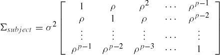
The covariance structure of the error is specified in the REPEATED statement. The SUBJECT = option specifies the independent random blocks and accordingly it defines the way the block diagonal matrix for all the errors is created. For example in our heart rate data for each of the twenty-four independent subjects there are four repeated measures. Hence the variance covariance matrix of the error vector ![]() is a diagonal matrix of twenty four blocks each of size 4 by 4, namely diag(Σsubject,...,Σsubject) where the 4 by 4 matrix Σsubject has an AR(1) covariance structure,
is a diagonal matrix of twenty four blocks each of size 4 by 4, namely diag(Σsubject,...,Σsubject) where the 4 by 4 matrix Σsubject has an AR(1) covariance structure,

and SAS provides an estimate of Σsubject using the estimation procedure indicated in the METHOD = option.
Example 6.4. Output 6.4
Analysis of Heart Rate Data

                      The MIXED Procedure
                   AR(1) Covariance Structure

                    Class Level Information

        Class     Levels  Values

        DRUG           3  ax23 bww9 control
        SUBJECT       24  1 2 3 4 5 6 7 8 9 10 11 12 13
                          14 15 16 17 18 19 20 21 22 23
                          24
        TIME           4  1 2 3 4


               REML Estimation Iteration History

       Iteration  Evaluations     Objective     Criterion

               0            1  403.36154087
               1            2  330.03350930    0.00002071
               2            1  330.03005861    0.00000000

                   Convergence criteria met.


                     R Matrix for SUBJECT 1

   Row          COL1          COL2          COL3          COL4

     1   32.28611617   26.52424845   21.79065925   17.90183919
     2   26.52424845   32.28611617   26.52424845   21.79065925
     3   21.79065925   26.52424845   32.28611617   26.52424845
     4   17.90183919   21.79065925   26.52424845   32.28611617
Covariance Parameter Estimates (REML)
Cov Parm Subject Estimate Std Error Z Pr > |Z|
AR(1) SUBJECT 0.82153729 0.04957930 16.57 0.0001
Residual 32.28611617 7.85162497 4.11 0.0001
Model Fitting Information for Y
Description Value
Observations 96.0000
Res Log Likelihood -242.206
Akaike's Information Criterion -244.206
Schwarz's Bayesian Criterion -246.637
-2 Res Log Likelihood 484.4117
Null Model LRT Chi-Square 73.3315
Null Model LRT DF 1.0000
Null Model LRT P-Value 0.0000
AR(1) Covariance Structure
Tests of Fixed Effects
Source NDF DDF Type III F Pr > F
DRUG 2 21 6.39 0.0068
TIME 3 63 15.85 0.0001
DRUG*TIME 6 63 13.34 0.0001
Compound Symmetry Structure
Tests of Fixed Effects
Source NDF DDF Type III F Pr > F
DRUG 2 21 5.92 0.0092
TIME 3 63 12.68 0.0001
DRUG*TIME 6 63 12.00 0.0001
Unstructured Covariance
Tests of Fixed Effects
Source NDF DDF Type III F Pr > F
DRUG 2 21 5.92 0.0092
TIME 3 21 15.82 0.0001
DRUG*TIME 6 21 21.91 0.0001 |
As shown in Output 6.4, for this data set the restricted maximum likelihood (REML) procedure converged in just two iterations. The REML estimate of Σsubject is ![]() (identified as the R matrix in SAS output) and is given by
(identified as the R matrix in SAS output) and is given by

The estimate of σ2 is ![]() =32.2861 and that of the AR(1) correlation parameter ρ is
=32.2861 and that of the AR(1) correlation parameter ρ is ![]() =0.8215. The respective asymptotic standard errors are
=0.8215. The respective asymptotic standard errors are ![]() = 7.8516 and
= 7.8516 and ![]() =0.0496.
=0.0496.
The tests for fixed effects, namely the variables DRUG and TIME, and TIME*DRUG, are shown next. The approximate F tests indicate that the interaction as well as DRUG and TIME effects are significant. For example, the TIME*DRUG interaction effect has the F statistic value 13.34 with 6 and 63 degrees of freedom and a p value 0.0001.
Suppose the chi-square test is used (program-output not shown) by specifying the CHISQ option in the MODEL statement, and the maximum likelihood estimation is implemented by using the option METHOD=ML in PROC MIXED statement. Then the chi-square statistic for testing TIME*DRUG interaction effect will have a chi-square statistic value 91.49 with 6 degrees of freedom and a p value 0.0001. The conclusions here are consistent with those observed using the mutivariate and univariate methods discussed in Chapter 5.
The univariate split-plot analysis under the model given in Equation 5.11 can be performed by adopting the option TYPE=CS in the REPEATED statement. The general (unstructured) covariance structure can also be adopted by using the option TYPE=UN. These options are also used in Program 6.4. The corresponding tests on fixed effects are presented in Output 6.4 for a comparison. A multivariate approach can also be taken as in Chapter 5 using PROC GLM. Of course, the tests used by PROC MIXED are different from multivariate tests. For example, for testing the TIME*DRUG interaction, the exact (for this example) F test corresponding to Wilks' Λ has the F statistic value 12.7376 with 6 and 38 degrees of freedom and a p value 0.0001, whereas the approximate F test in MIXED procedure has an F statistic value of 21.91 with 6 and 21 degrees of freedom and a p value 0.0001. The conclusions are however the same.
A few brief comments about the preference for the covariance structure are in order. To choose a covariance structure among the three used here, we may look at AIC and BIC values produced in the output of PROC MIXED. These are reported in the following table.
| Covariance | AIC | BIC |
| AR(1) | −244.206 | −246.637 |
| CS | −245.917 | −248.348 |
| UN | −248.758 | −260.912 |
Since the values of AIC and BIC are both maximum for the AR(1) structure, this structure seems to be most appropriate among the choices considered in the above table.
6.5.2. Unbalanced and Unequally Spaced Data
Unbalanced and unequally spaced data occur in practice due to many factors. These data are especially common in clinical experiments where patients reschedule their appointments and/or drop out. Additionally, many consumer preference surveys, where two or more groups of consumers are asked to try out the products over time, and then report their preferences will also yield such data. The techniques illustrated here are useful when there is a reason to believe that the dropouts are fairly random. In cases, when there is some nonrandom assignable cause for the dropouts, the techniques given here are not applicable. See Little and Rubin (1987) for details on appropriate techniques for such data sets.
EXAMPLE 5
Fitting Markov Structure, Audiology Data The data are the percentage of correct scores on a sentence hearing test administered to two groups of subjects wearing two different cochlear implant types denoted by A and B respectively. There are 19 subjects in group A and 16 subjects in group B. The hearing tests are administered 1, 9, 18, and 30 months after the implantation of the devices. The objective of the study is (i) to determine if there is any difference between the two cochlear implants and also (ii) to determine the average improvement curves as functions of the length of time since implantation. The raw data have several missing values and are observed at unequally spaced time points.
Suppose we decide to fit two different quadratic functions for different groups, as functions of time since implantation, for the scores on the hearing tests. For the uth individual in the ith group, i = 1,2, we consider the following model relating the improvement as a function of TIME,
time = t1, t2, t3, t4; i = 1,2; u=1,...,ni, n1=19, n2=16. We assume that ϵiu are all independently distributed as N(0,σ2), β0i are all independently distributed as N(0,σ2), β0i are also independent of each other for i = 1,2; u=1,...,ni. The coefficients β1i and β2i, i =1,2 allow the curves for the two groups to be different in their linear and quadratic time components. Thus corresponding terms in Program 6.5 represent the linear and quadratic interactions of TIME with the group effect GP. We also assume that the variance covariance matrix of the piu repeated measurements, collected on a given subject over time since the implantation of the hearing device, is given by

where for our data t1=1, t2=9, t3=18, and t4=30. The above covariance structure is often referred to as the Markov covariance structure and is especially useful in modeling spatial correlations. Since this covariance structure involves the powers of the parameter ρ, it is also referred to as the spatial power covariance structure. To fit this covariance structure the appropriate TYPE = option in the REPEATED statement is SP(POW)(TIME1), where TIME1 is the variable taking values as the actual time points for which the data were observed (in our example these are 1, 9, 18, and 30 respectively). Program 6.5 is used to analyze the audiology data. Output 6.5 follows.
/* Program 6.5 */
options ls=64 ps=45 nodate nonumber;
    title1 'Output 6.5';
    data aud;
    infile 'audiology.dat';
    input gp$ y1-y4;
    data aud;
    set aud;
    array t{4} y1-y4;
    subject+1;
    do i = 1 to 4;
    if (i = 1) then time=1;
    if (i=2) then time=9;
    if (i=3) then time=18;
    if (i=4) then time=30;
    time1=time;
    y=t{i};
    output;
    end;
    drop i y1-y4;
    run;
title2 'Fit Different Quadratic Curves for Groups A and B';
proc mixed data=aud_n method=reml covtest;
class gp subject;
model y= gp time time*gp time*time time*time*gp/htype=1;
repeated/type=sp(pow)(time1) subject=subject r;
run;
title2 'Common Quadratic Term for Groups A and B';
proc mixed data=aud_n method=reml covtest;
class gp subject;
model y= gp time time*gp time*time;
repeated/type=sp(pow)(time1) subject=subject r;
run;
title2 'Common Linear and Quadratic Terms for Groups A and B';
proc mixed data=aud_n method=reml covtest;
class gp subject;
model y= gp time time*time/s;
repeated/type=sp(pow)(time1) subject=subject r;
run;
title2 'Common Quadratic Curve for Groups A and B';
proc mixed data=aud_n method=reml covtest;
class gp subject;
model y= time time*time/s;
repeated/type=sp(pow)(time1) subject=subject r;
run;Some explanation is needed about the MODEL statements used in Program 6.5. Since for each of the two groups (GP) the two models will have different coefficients, we introduce a CLASS variable GP and incorporate that in the model along with linear and quadratic components of the interaction with TIME. These are denoted by GP, TIME*GP, and TIME*TIME*GP respectively. If any of these are found to be statistically not significant the corresponding terms can perhaps be dropped in the process of finalizing the model. Further, the curves for the two groups will be deemed parallel if both of the interactions TIME*GP and TIME*TIME*GP are zero. Additionally, if a common quadratic curve can be fitted it will amount to saying that the two curves are identical and the GP effect is also absent.
The acceptance of the null hypothesis
indicates that a common quadratic term can be fit for the two groups. Since the polynomial growth curves are fit in a sequence, TYPE I sums of squares can be utilized to test this hypothesis. The SAS code for testing this hypothesis is provided in the first MODEL statement in Program 6.5. From Output 6.5, we see that the approximate p value computed for the F statistic using the TYPE I sum of squares is 0.8508. Under H0, F follows an F-distribution with (1, 71) degrees of freedom. The observed value of F=0.8508 is not significant at any reasonable level of significance. Hence we do not reject H0(1). Thus a common quadratic term can be used for the two groups.
Given that the two groups have common quadratic terms, acceptance of the null hypothesis
implies that the two groups have parallel quadratic improvement curves. That is, these two growth curves are possibly different only in their intercept terms. The intercept for the two groups are respectively β0+β01 and β0+β02. The second MODEL statement in Program 6.5 tests this hypothesis which has been formally expressed as H0(2). From Output 6.5, the p value for test is 0.6649. Thus H0(2) is not rejected.
Finally, not rejecting the hypothesis
implies that a common quadratic improvement curve fits both the groups. The third MODEL statement in Program 6.5 tests H0(3). Since the p value for testing H0(3), given that the quadratic curves are parallel, is 0.1514 this hypothesis is not rejected as well.
Example 6.5. Output 6.5
Fit Different Quadratic Terms for Groups A and B
                     Tests of Fixed Effects

           Source         NDF   DDF  Type I F  Pr > F

           GP               1    33      2.23  0.1453
           TIME             1    71     64.20  0.0001
           TIME*GP          1    71      0.20  0.6533
           TIME*TIME        1    71     33.43  0.0001
           TIME*TIME*GP     1    71      0.04  0.8508


            Common Quadratic Term for Groups A and B
                    Tests of Fixed Effects

           Source      NDF   DDF  Type III F  Pr > F

           GP            1    33        1.32  0.2581
           TIME          1    72       85.48  0.0001
           TIME*GP       1    72        0.19  0.6649
           TIME*TIME     1    72       33.85  0.0001


      Common Linear and Quadratic Terms for Groups A and B
                  Solution for Fixed Effects

    Effect     GP      Estimate     Std Error    DF       t

    INTERCEPT       15.36207906    5.81203232    33    2.64
    GP             a   11.05462289    7.52633962    33    1.47
    GP             b    0.00000000             .     .       .
    TIME             2.87736050    0.30970055    73    9.29
    TIME*TIME       −0.05748638    0.00983687    73   -5.84


                   Solution for Fixed Effects

                   Pr > |t|

                     0.0125
                     0.1514
                          .
                     0.0001
                     0.0001
Tests of Fixed Effects
Source NDF DDF Type III F Pr > F
GP 1 33 2.16 0.1514
TIME 1 73 86.32 0.0001
TIME*TIME 1 73 34.15 0.0001
Common Quadratic Curve for Groups A and B
Solution for Fixed Effects
Effect Estimate Std Error DF t Pr > |t|
INTERCEPT 21.32088661 4.20808393 34 5.07 0.0001
TIME 2.88426715 0.31011367 73 9.30 0.0001
TIME*TIME −0.05773884 0.00984910 73 -5.86 0.0001
Tests of Fixed Effects
Source NDF DDF Type III F Pr > F
TIME 1 73 86.50 0.0001
TIME*TIME 1 73 34.37 0.0001 |
Having eliminated the possibility of any differences between the two model we fit a common quadratic curve for the two groups using the last MODEL statement of Program 6.5. As seen from the bottom part of Output 6.5, the common quadratic curve ![]() fits well to the data, where
fits well to the data, where ![]() =21.3209,
=21.3209, ![]() =2.8843 and
=2.8843 and ![]() =−0.0577. Since
=−0.0577. Since ![]() is positive and
is positive and ![]() is negative, this curve which, representing the effectiveness of implantation over a period of time, increases initially, stabilizes, and slowly decreases after a period of time.
is negative, this curve which, representing the effectiveness of implantation over a period of time, increases initially, stabilizes, and slowly decreases after a period of time.