3
Aerodynamic Performance Analysis of Three Different Unmanned Re‐entry Vehicles
Giuseppe Pezzella1 and Antonio Viviani2
1 Italian Aerospace Research Centre, Capua, Italy
2 University of Campania 'Luigi Vanvitelli', Aversa, Italy
3.1 Introduction
This chapter deals with the aerodynamic performance analysis of three reusable and unmanned aerial vehicles conceived as flying laboratories to perform experimental flights in low Earth orbit (LEO). Each vehicle concept is an orbital re‐entry vehicle (ORV), with re‐entry energy of the order of 25 MJ/kg. They are flying test beds (FTBs) that will re‐enter the Earth’s atmosphere, thus allowing tests of critical re‐entry technologies to be performed. The primary objective is to test in real flight conditions various thermal protection systems (TPSs) and hot structures that are potential candidates for next‐generation re‐entry vehicles. The secondary objective is to provide system‐design tests of such re‐entry vehicles, to address controlled gliding re‐entry and to validate know‐how related to in‐flight measurement techniques.
Besides these objectives, they will also gather the aerothermal data needed to improve wind tunnel test facilities (including plasma wind tunnel facilities) and computational fluid dynamics (CFD) predictions and transpose them to flight. In particular, the vehicle will provide aerodynamic and aerothermodynamic flight data to correlate with ground testing results, such the ‘Scirocco’ plasma wind tunnel at CIRA1), thus providing new insights into the complex aerothermodynamic phenomena and improving prediction methodologies and their extrapolation to flight capabilities.
Based on experience in experimental vehicles, a progressive flight demonstration approach is preferable, since this limits the risks, allows progressive investment efforts, and ensures that more challenging developments benefit from results and findings obtained through a systematic approach.
So far, Europe has undertaken the development of three very different FTBs: namely ARD (Atmospheric Re‐entry Demonstrator), EXPERT (European Experimental Reentry Testbed) and IXV (Intermediate Experimental Vehicle).
ARD was a scaled‐down version of an Apollo capsule. It was launched by ARIANE 5 V503 on October 21, 1998 [1]. After a successful sub‐orbital and re‐entry flight, it was recovered in the Pacific Ocean. ARD allowed an assessment of the aerodynamics of this kind of capsule, which is still a very attractive design solution for manned high‐energy re‐entry, such as return from Mars or Moon missions [2].
EXPERT, which has not yet flown, is a small sphere‐cone FTB designed for in‐flight testing of advanced TPSs, wall catalyticity, flow transition assessments, and so on [3].
Finally, the Intermediate Experimental Vehicle is shown in Figure 3.1. It is a rather blunt FTB that features a lifting‐body configuration [4]. It was tested in re‐entry flight conditions on 11 February 2015 at the end of a sub‐orbital flight that had an energy level very close to that of an orbital re‐entry [5].

Figure 3.1 The IXV.
IXV performed several in‐flight experiments, such as the guidance, navigation and control (GNC) of a flapped lifting‐body aeroshape and TPS catalyticity. A description of the aerodynamic and aerothermodynamic characterization of IXV can be found in the literature [4, 5].
The FTBs developed so far are capsules and lifting‐body vehicles only. Therefore, in a step‐by‐step approach with increasing levels of complexity, only winged‐body configurations have so far been explored, as discussed in this chapter.
A reusable ORV operates in different flight regimes from subsonic to hypersonic speeds. A typical mission profile includes:
- ascent phase, where the spacecraft is attached to a launch vehicle and flown to altitude;
- orbit phase, where the vehicle orbits in space until completion of its mission;
- descent phase, where the ORV re‐enters the atmosphere and lands like a conventional airplane for subsequent use.
During the descent the spacecraft encounters several flowfield regimes (rarefied, transitional, and continuum flow) and speeds of flow (hypersonic, supersonic, transonic, and subsonic). Therefore, the choice of vehicle aeroshape and its aerodynamic characterization in different flight conditions is fundamental for its safe return and mission success. Usually, the vehicle configuration is continuously adapted throughout the design phase by means of a trade‐off study (a ‘multidisciplinary design optimization’) involving several competing ideas for meeting the mission requirements under the design constraints. For example, the vehicle concept will have to be carried to low‐Earth orbit using a small launcher. It must then re‐enter the atmosphere, allowing a number of experiments on critical re‐entry technologies to be performed, before descending from a hypersonic regime down to landing. Figure 3.2 shows some wing–body configurations that might meet these requirements [6].

Figure 3.2 FTB trade‐off configurations.
The configurations differ in terms of features such as planform shape, cross section, nose camber, wing‐swept angle and vertical empennages. Of course, the winning configuration from the aerothermal point of view is the one with simultaneously the best aerodynamic and aerothermodynamic performance. The current most promising vehicle configurations according to the trade‐off analyses, are shown in Figures 3.3–3.6. The different shapes of the side views are shown in Figure 3.3, ranging from blunt to sharp.

Figure 3.3 ORV‐WSB body configurations: top, rather blunt; middle, sharp; bottom, spatulared.
Figure 3.4 shows the sharp vehicle configuration, named ORV‐WSB. It is also shown docked with a service module with its solar panels deployed [6, 7].

Figure 3.4 ORV‐WSB configuration in flight and docked to a service module with solar panels.
The blunt configuration, ORV‐WBB, is shown in Figure 3.5 [7].

Figure 3.5 Rather blunt vehicle configuration.
Finally, Figure 3.6 displays the spatular‐body (SB) configuration, ORV‐SB [7].

Figure 3.6 The spatular body configuration.
This shape is most attractive, being the only viable way to integrate scramjet propulsion (see Box 3.1) in the vehicle’s aerodynamic configuration (see Figure 3.7, where the ORV‐SB features a scramjet engine on the belly side), thus evolving towards a waverider aeroshape [8].

Figure 3.7 The spatular body configuration with scramjet.
So, all ORV concepts belong to the wing–body vehicle class. Such configurations, however, differ in terms of nose camber, planform shape, cross section, wing‐swept angle and vertical empennages. These differences in aeroshape can be seen in Figure 3.11, where each configuration is superimposed.

Figure 3.11 ORV aeroshapes comparison.
These aeroshapes are conceived in such a way as to allow the ORV to re‐enter the Earth’s atmosphere with an aerodynamic efficiency that is better than the Space Shuttle, which had a maximum L/D ratio of about 1. The ORV will fly a re‐entry trajectory with a long‐endurance leg in the upper atmosphere, using ‘low’ (with respect to the Shuttle guidance approach) and modulated AoA guidance. This brings a number of benefits, such as:
- overcoming the critical heat flux region in a quasi‐thermal equilibrium condition, ensuring that the internal temperature remains less than the peak temperature that a steep re‐entry can produce
- exposing small parts of the vehicle to a high heat flux (these are protected with an advanced TPS such as ultra‐high‐temperature ceramics), but leaving most of it exposed to a lower heat flux, allowing the use of simpler, cheaper, and lighter materials.
The aerodynamic performance of these ORVs, from the hypersonic down to subsonic regime, can be assessed. With this in mind, both low‐order methods (hypersonic panel methods) and CFD design analysis have been considered in accordance with a phase‐A design level.
The work is currently at an early design stage, so low‐order methods are extensively used. CFD simulations are performed only to address the reliability of the low‐order method design results and to investigate complex flowfield phenomena that are not predictable with simplified tools [10, 11, 12].
Both perfect gas and thermochemical non‐equilibrium CFD simulations are performed at several points of the flight scenario in the range between Mach 0.3 and Mach 25. In the reacting gas computation, the air is modelled as a mixture of five species (O2, N2, NO, N, and O). An analysis of the longitudinal‐ and lateral‐directional stability was also provided for one concept, together with the main interesting features of the flowfield past the vehicles at Mach numbers where real‐gas effects occur. In fact, it is well known that the pitching moment can be highly modified by high‐temperature real gas effects, thus affecting vehicle’s stability and trimming conditions [13].
3.2 Vehicle Description
The vehicle concepts considered here feature a compact wing‐body configuration equipped with a rounded‐edge delta‐like fuselage cross section, a delta wing, and a V‐tail. The vehicle architecture shows a blended wing body (BWB) interface and a flat‐bottomed surface to increase its overall hypersonic performance. The fuselage was designed to be longitudinally tapered, in order to improve aerodynamics and lateral‐directional stability, and with a cross section large enough to accommodate all the vehicle subsystems such as, for example, the large propellant tanks for long missions.
This has a large impact on vehicle performance. From the aerodynamic point of view, the lift and the aerodynamic efficiency are mainly determined by the fuselage fineness and by the shape of the vehicle cross section [16]. The forebody is characterized by a rather simple cone–sphere geometry with smooth streamlined surfaces on the upper and lower side of fuselage, and by the nose drop‐down configuration, typical of winged hypersonic vehicles. The nose camber is low enough to reduce the elevon size in order to provide the desired trim range with elevon deflections, and also to improve internal packaging of the vehicle’s subsystems. The wing size and location were defined using trade‐off studies so as to improve vehicle aerodynamics and to provide static stability and controllability during flight [10, 17].
The wing is swept back to optimise performance with respect to supersonic drag and aerodynamic heating. A properly designed strake could be added in the future, depending on the specific landing requirements. A wing dihedral angle of 5° is also provided to enhance lateral‐directional stability. The wing also features a high length‐to‐width ratio to minimise drag, a section shape that is maintained from root to wing tip, and a nearly flat‐bottomed surface to efficiently dissipate aeroheating. The vertical tails’ sweep angle is 45°. Control power for the vehicle is provided by two wing‐mounted elevon surfaces (which must serve as ailerons and elevators), and rudders. Used symmetrically, the elevons are the primary controls for pitch motion. Roll control is obtained through asymmetrical usage of the elevons. Rudders help to provide directional control, while vertical tails allow for sideslip stability. During entry, when the vehicle is flying at high AoAs, the rudders should be augmented by the RCS. For example, Figure 3.14 shows the ORV‐WSB concept with RCS pods on the base. Arrows indicate the thrust provided by each pod. Therefore, by appropriately combining the thrust vectors it is possible to control pitch, roll and yaw.
Figure 3.14 ORV‐WSB dihedral angles with RCS pods on base.
The vehicle may be provided by a body flap located at the trailing edge of the fuselage in order to augment pitch control and to shield the nozzle of the propulsion subsystem (see the image of ORV‐WBB in Figure 3.5). Trim capability to relieve elevon loads is obtained by body‐flap deflection. At hypersonic speeds, a surface behind the vehicle CG balances the nose‐up pitching moment typical of this configuration at hypersonic speeds.
Finally, the aerodynamic control surfaces are designed to be large enough to provide stability without sacrificing too much lift.
3.3 Flight Scenario and Flow‐regime Assessment
It is planned that the ORV should perform a complete re‐entry flight from LEO orbit at 200 km. The return trajectory is based on a different strategy, from the guidance point of view. The vehicle will be held as long as possible in the highest level of the atmosphere that is compatible with the thermal constraints of the descent.
It has better gliding re‐entry and a high‐manoeuvring capabilities than the reference re‐entry of the Space Shuttle, characterized by moderate AoAs (up to 20°). Longer flight durations are possible, allowing for more extended in‐flight testing capabilities in high‐energy hypersonic flight conditions.
In the framework of flight mechanics trade‐off analyses, several re‐entry trajectories have been computed, thus defining the vehicle flight envelope needed to address vehicle aerodynamics. For example, Figure 3.15 and Figure 3.16 show a number of re‐entry trajectories evaluated supposing that the vehicle heat flux constraint ranges between 1.1 and 2 MW/m2 and that the dynamic pressure limit is equal to 12 kPa. The Mach–Reynolds numbers grid in the altitude–velocity map of Figure 3.16 characterizes the vehicle aerodynamics according to the space‐based design approach [18].

Figure 3.15 ORV re‐entry: top, time history of light envelope; bottom, AoA profiles.

Figure 3.16 ORV re‐entry: top, velocity–altitude map; bottom, time history of stagnation point heat flux profiles.
The time at which re‐entry is ended – close to about 5000 s – is larger than for a conventional re‐entry in, for example, the Space Shuttle. Note that for each trajectory shown in Figure 3.15 and Figure 3.16 the guidance technique is the same, but the AoA profiles are different (see Figure 3.15). Typically, the more common approach to the definition of the guidance strategy makes use of a predefined AoA profile, characterized by high values for the most critical re‐entry phase, during which the heat flux is critical for vehicle safety. The bank angle control is usually applied in such a way that the flight path can follow a predefined drag–velocity profile and create the required cross‐range.
An alternative approach has been adopted here, in order to be compliant with the specific ORV project requirements. This involves modulating the AoA profile during the re‐entry critical phases. The AoA will be set as close as possible to the one corresponding to the maximum efficiency (at least in the ‘dense’ atmosphere range) that is compatible with the maximum heat flux the vehicle (TPS and cold structure) can sustain. This kind of AoA guidance profile should allow for greater vehicle manoeuvrability along the trajectory and will expose a smaller part of the vehicle to the higher heat flux, thus allowing for a TPS mass reduction and increasing the mission’s safety level. For instance, the optimized long‐endurance trajectories are characterized (for a relevant part of the trajectory) by a quasi‐steady thermal equilibrium condition near the maximum admissible heat flux value at the stagnation point (see Figure 3.16, bottom), thus taking advantage of radiative cooling.
As far as flight‐regime assessment is concerned, it is worth noting that along with the atmospheric re‐entry trajectory, going from upper to lower altitudes, the vehicle experiences three main flow regimes. They are:
- the hypersonic–supersonic regime, in the upper part of the descent
- the transonic and subsonic regimes, in lower atmospheric layers.
At hypersonic‐speed flow, three main (and heavily overlapping) regimes apply. They are:
- the rarefied‐transitional regime, on the one hand, and
- the viscous‐interaction regime and
- the real‐gas regime, on the other hand, which lie in the continuum flow regime.
Consequently, knowing where in the re‐entry trajectory each of these flight regimes is established is extremely important in order to address vehicle performance. For example, it is well‐known that real‐gas and viscous effects play a significant role in the vehicle’s aerodynamics (drag rise and trim conditions) and aerothermodynamics. This means that vehicle design demands different
- flow models, ranging from a perfect gas to a reacting gas mixture
- flowfield solution approaches, ranging from DSMC to Navier–Stokes with and without slip flow conditions
to provide a full description of key flow phenomena affecting the vehicle’s aerodynamic and aerothermodynamic characteristics.
3.4 Rarefied and Transitional Regimes
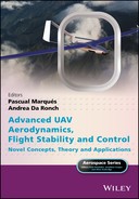
Once the vehicle has started its descent, the atmospheric density is low enough that the continuum assumption breaks down. Since individual molecular collisions are important, one must consider the general microscopic mass, force and energy‐transfer problem at the vehicle surface. In these conditions, there are two distinct subregimes: the re‐entry through the upper part of the atmosphere and that through the lower part of the high atmosphere. In the former, the free molecular flow (FMF) regime is completely established, while in the latter the transitional flow regime (TFR) applies. Of course, the limit between these two flow conditions depends on altitude and vehicle dimensions. For instance, the similarity parameter that governs these different flow regimes is the Knudsen number (rarefaction parameter), defined as:
where λ is the molecular mean‐free path, Lref is the characteristic length of the body and γ is the specific heat ratio [13, 17]. Indeed, when the air density becomes rarefied enough the molecular mean‐free path can become as large as the scale of the body itself. This condition is indeed known as FMF regime. Here, the aerodynamic characteristics of the vehicle are determined by individual, scattered molecular impacts, and must be analysed on the basis of kinetic theory. Because of this, several particle simulations, such as DSMC analyses, are mandatory. FMF conditions result in an abrupt loss of vehicle aerodynamic efficiency due to a suddenly increase of drag and lift drop. Further down in the atmosphere (in other words, higher λ) the TFR is established. The DSMC approach is still valid but demands high computational effort to simulate the increasing number of molecules. Fortunately, in these flow conditions the slip conditions and temperature jump can be introduced in the continuum approach (in other words, a Navier–Stokes approximation) to take into account for the rarefaction effects.
The rarefied and transitional regimes for ORV concepts are shown in Figure 3.17.
Figure 3.17 ORV re‐entry scenario in the Mach–Reynolds map with iso‐Knudsen curves.
The ORV re‐entry trajectory is reported in the Mach–Reynolds numbers map together with iso‐Knudsen curves, which bound the different flow regimes, according to the Bird regime classification. As one can see, the region for 10−3 < Kn∞ < 10 is the transitional flow region. Therefore, above about 200 km altitude the ORV is in the FMF (in fact, Kn∞Lref ≈ 70); while from the entry interface (in other words 120 km, the red square in Figure 3.17) to about 87 km (green rhombus in Figure 3.17) the vehicle is in the TFR.
Finally, after that, continuum flow conditions are established.
3.5 Viscous‐interaction Regime
It is the flow regime where, due to low Reynolds number and high Mach number effects, the boundary layer and the shock layer merge into a viscous shock layer enveloping the vehicle. This results in a loss of ORV aerodynamic performance assuming that the vehicle drag in this regime rises, thus lowering spacecraft aerodynamic efficiency.
The viscous interaction regime (VIR) is defined by the hypersonic viscous interaction parameter (VIP):

where

and
By using the reference enthalpy approach to account for compressibility effects, an estimation of the VIR extension for the ORV can be found (Figure 3.18). This shows the vehicle re‐entry trajectory both by means of an altitude‐vs‐Mach curve and a Mach‐vs‐VIP curve. As shown, two boundaries are also reported in the figure according to the criterion chosen in the past to address the VIR for the Space Shuttle. Therefore, very roughly one can conclude that for the ORV the VIR ranges from about 60 to 83 km altitude, close to the boundary of 86 km highlighted above as the beginning of the transitional flow regime.

Figure 3.18 ORV re‐entry trajectory in the Mach/altitude‐viscous parameter map.
3.6 High‐temperature Real‐gas Regime
The equilibrium/non‐equilibrium real‐gas regime is characterized by relatively high‐density and high‐velocity flow conditions. For instance, the hottest thermal environment is encountered and many chemical reactions occur. Therefore, the modelling of such phenomena requires enforcing the Navier–Stokes equations with input data such as chemical equilibrium constants and reaction rates for the reaction mechanisms involving all the species that compose the gas mixture at the specified flight conditions.
In this framework, the current ORV nominal re‐entry trajectory is illustrated in Figure 3.19 in an altitude–velocity map, where real‐gas phenomena that occur during re‐entry and which are relevant for assessing the vehicle aerodynamics and aerothermodynamics are shown [13].

Figure 3.19 ORV re‐entry scenario in the altitude–velocity plane with real gas map.
For instance, Figure 3.19 highlights that when the ORV vehicle is flying at 6 km/s at about 70 km altitude, oxygen is completely dissociated because the velocity is larger than that corresponding to the O2‐dissociated domain. On the other hand, nitrogen begins to dissociate because we are near the green dashed line which represents the N2 10% dissociation boundary. Indeed, the high‐energy of re‐entry flows leads to strong heating of the air in the vicinity of vehicle. Depending on the temperature level behind the bow shock wave (in other words, depending on the flight velocity), the vibrational degrees of freedom of the air molecules are excited and dissociation reactions of oxygen and nitrogen molecules may occur.
The high‐temperature real‐gas effects described here are enabled by energy transfer from the translational energy stored in the random motion of the air particles, which is increased by the gas heating up, to other forms of energy. Because this energy transfer is brought about by air particle collisions, it requires a certain time to happen. The time required to reach equilibrium is defined by the local temperature and density. Therefore, depending on the ratio of the relaxation time to a characteristic timescale of the flow, the chemical and thermal relaxation processes can be non‐equilibrium, in equilibrium or frozen flow, thus influencing the vehicle’s aerodynamic and aerothermodynamic performance. For example, flow thermochemical conditions influence vehicle pitch trim and aeroheating loads along with the re‐entry flight.
The similarity parameter that governs the thermochemical regimes is the Damkohler (Da) number, defined as:

where the characteristic flow time of particles passing a region of the flow tc is usually the ratio of the characteristic dimension L (the shock stand‐off distance for instance) and the velocity u; the relaxation time refers to both chemical reactions (in other words chemical relaxation) and internal degrees of freedom of the flow molecules: vibration, rotation and so on (in other words thermal relaxation) [19]. Therefore,

So, for chemical reaction the Damkohler number reads:

where nk and ![]() represent the number density and the chemical production rate of species k, respectively [19].
represent the number density and the chemical production rate of species k, respectively [19].
For thermal relaxation we can define the Damkohler as

where τv is the vibrational relaxation time, usually described by the Landau–Teller approximation for harmonic oscillators, which is valid to about 5000 K [19]. As a result, the chemical and thermal regimes may be loosely defined as follows:
| Da = 0 | chemically/thermally frozen |
| 10−2 < Da < 103 | chemical/thermal non‐equilibrium flow |
| Da = ∞ | chemical/thermal equilibrium. |
At very high altitudes where the densities are very small or at low speeds where temperatures are low, reaction rates are slow compared to the hydrodynamic timescales (Da << 1). This enables the frozen flow assumption to be used and solutions are restricted to those that model the flow of a multi‐component fluid as a continuum (or free‐molecular) problem with an appropriate equation of state and real (in other words, temperature‐dependent) thermodynamic data.
On the other hand, at low altitudes the densities are high and the flow is likely to be characterized by fast chemical reactions with short timescales compared to the fluid velocity (Da >> l). In this regime the assumption of equilibrium chemistry in the shock layer is more appropriate.
In the mid‐range density regime, the assumption of either frozen or equilibrium flow, whilst accurate in some portions of the shock layer, would lead to over‐ (frozen) or under‐ (equilibrium) prediction of temperature in other areas [13, 17]. In reality, between these two regimes the density is such that the flow cannot be accurately characterized as being either frozen or in chemical equilibrium. It is in this flight region that non‐equilibrium chemical kinetics must be considered [19].
Figure 3.19 also suggests that there will be an increasing number of species in the different domains along the descent trajectory. Therefore, accurate CFD simulations must rely on a flow thermochemical model appropriately tuned on the base of the free‐stream conditions of the trajectory point to simulate.
This discussion suggests that, due to the continual exchange of energy between the transitional and internal degrees of freedom of the flow molecules, the air at hypersonic speeds results in a mixture in thermal and/or chemical non‐equilibrium in the different domains of the altitude–velocity map, as shown in Figure 3.20 and Tables 3.1 and 3.2.

Figure 3.20 Re‐entry scenario in the altitude–velocity plane with the stagnation point flow regimes and thermochemical phenomena. Refer to main text for key.
Table 3.1 Regions with their expected aerothemal phenomena.
| Region | Aerothermal phenomena |
| A | Chemical and thermal equilibrium |
| B | Chemical non‐equilibrium with thermal equilibrium |
| C | Chemical and thermal non‐equilibrium |
Table 3.2 Chemical species in high‐temperature air.
| Region | Model | Species |
| I | 2 species | O2, N2 |
| II | 5 species | O2, N2, O, N, NO |
| III | 7 species | O2, N2, O, N, NO, NO+, e− |
| IV | 11 species | O2, N2, O, N, NO, NO+, O+2, N+2, O+, N+, e− |
This figure provides several insights into the trends expected in the air chemistry of the flight stagnation region of the ORV forebody. For instance, Figure 3.20 shows three different regions:
- A is the region of chemical and thermal equilibrium.
- B is the region of chemical non‐equilibrium and thermal equilibrium.
- C is the region of chemical and thermal non‐equilibrium.
Using Table 3.1, one can rapidly assess the most likely thermochemical model for the high‐fidelity CFD simulation once trajectory freestream conditions are known.
3.7 Laminar‐to‐turbulent Transition Assessment
During descent from suborbit or orbit, re‐entry vehicles experience transition from fully laminar to fully turbulent flow conditions. In the latter case, both aerodynamic drag and an aeroheating increase must be accounted for in the vehicle design [20]. Therefore, a critical aeroheating design issue for all aerospace vehicles is to assess in what region of the descent flight trajectory the boundary‐layer transition (BLT) occurs and to determine the corresponding increase in heat transfer/surface temperature.2
To avoid the worst case scenario from an aeroheating perspective, BLT needs to occur well past the region of peak heating on the trajectory (in other words, the region where the product of freestream density and velocity to the third power is a maximum) [14, 15]. Thus, a reasonably accurate determination of flight conditions where BLT occurs is essential for most aerospace vehicles, in order to ensure that aeroheating levels and loads remain within TPS design limits. Ideally, such information would be incorporated into the design of the TPS, including material selection, the split line definition, and choice of material thickness.
Although progress has been made in developing computational techniques for predicting hypersonic BLT onset, aerothermodynamicists still rely primarily on semi‐empirical methods based on local flow conditions, such as local Mach and Reynolds numbers. For example, for the Shuttle Orbiter and other vehicles, an empirical correlation for hypersonic transition – the transition criterion based on the parameter Reθ/Me:

was developed [13,14,15]. Here, Reθ is the momentum thickness Reynolds number and Me is the boundary‐layer edge Mach number. Advances in numerical (in other words CFD) flowfield solutions and the phosphor thermography technique in wind tunnel experiments have given such approaches a boost.3
In practice, CFD results provide local conditions of interest about the model, specifically boundary layer thickness, Me, and Reθ at the location of the surface disturbance(s). Through experimental investigations, designers try to correlate the value assumed by the parameter Reθ/Me to the transition front detected in the wind tunnel.
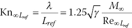
Because the assessment of the local flow conditions demands accurate CFD computations, which are, of course, not compliant with a phase‐A design level, a transition method based on freestream Reynolds (Re∞) and Mach (M∞) numbers has been adopted. For example, Figure 3.26 reports the transitional Reynolds limit evaluated by means of the following transition criterion:
where ReT and Cm depend on the type of flow, flying AoA, leading‐edge sweep angle, and leading‐edge nose bluntness [21]. As shown, the transition criterion highlights that, below about 46 km, altitude turbulent‐flow conditions are expected.
![Graph of time to re-entry [s] vs. log reynolds [–] displaying 3 intersecting curve plots for freestream reynolds, transition re limit, and altitude.](http://images-20200215.ebookreading.net/13/1/1/9781118928684/9781118928684__advanced-uav-aerodynamics__9781118928684__images__c03f026.gif)
Figure 3.26 Assessment of laminar‐to‐turbulent transition.
3.8 Design Approach and Tools
A review of the aerodynamic analyses needed for the development of the aerodynamic database (AEDB) of the vehicle concept is now performed. These evaluations are aimed only at creating a preliminary AEDB, compliant with a phase‐A design level [22,23,24]. The goal is to provide aerodynamic characteristics for flight‐mechanics and thermal‐shield design analyses. It must be verified that vehicle, after the de‐orbit manoeuvre, is able to stay within the load constraints (in other words, entry corridor) when flying trimmed during descent to a conventional runway landing.
The AEDB is prepared as a function of Mach number, AoA, sideslip angle, aerodynamic control surface deflections, and Reynolds number, according to the space‐based design approach [18]. This design approach dictates the generation of a complete dataset as function of a number of independent parameters (in other words, M∞, Re∞, α, β) as shown in Figure 3.27.

Figure 3.27 Space‐based design approach in the altitude–velocity map.
An accurate aerodynamic analysis of all these flight conditions, however, is very complex and time consuming, and is not compatible with a Phase‐A design study, in which fast prediction methods are mandatory.
In the preliminary design phases, the evaluation of the vehicle AEDB is mainly accomplished by means of engineering tools, and a limited number of more reliable CFD computations (continuum regime only), according to the workflow shown in Figure 3.28 [22,23,24,25].

Figure 3.28 Tools and methods.
CFD computations are performed in order to verify the accuracy of the design results and to focus on some critical design aspects not predictable with simplified tools. This overall process is referred to as ‘anchoring’ of the engineering‐level methods. The anchoring process permits a few select CFD solutions to be used beyond the specific flight conditions in which they were original run.
The anchoring process also allows for the cost‐effective use of high fidelity, and computationally expensive, CFD solutions early in the design process, when the vehicle trajectories are often in a constant state of change [26, 27]. The CFD anchoring ‘space’ is defined by a small number of CFD solutions in Reynolds‐Mach‐AoA space, as shown in Figure 3.29.

Figure 3.29 Hypothetical CFD anchoring mesh in Reynolds‐Mach‐AoA space.
Note that CFD analysis is nevertheless essential in preliminary design studies, keeping in mind the limited capability of an engineering‐based approach in modelling complex flow interaction phenomena and aerodynamic interference, such as shock–shock and shockwave boundary‐layer interactions.
Experience shows that an aerodynamic configuration that seems to be promising when evaluated by simplified methods is not always a feasible solution after performing more detailed calculations. But every layout deemed infeasible by the preliminary aerodynamic examination has no reasonable chance of realization. Therefore, the approach implemented in the engineering‐based approach is fully justified, as it is much easier and more rapid, and hence the assessment of rearrangements can be done extremely quickly.
As a result, ORV aerodynamics in FMF conditions have also been provided with low‐order methods. In the transitional flow regime (the one bridging the continuum and the free molecular regimes) the bridging relationships approach is applied.
Finally, in the continuum flow regime, vehicle aerodynamic appraisal is performed with both low‐order and CFD methods.
All aerodynamic data are provided in a format that will allow a build‐up from a basic configuration, by means of contributing elements to each force or moment component such as control surface effectiveness, and so on. Data are presented in a manner that treats each force and moment separately to facilitate the build‐up procedure. Engineering codes are used for initial screening of aerospace vehicle concepts, trade studies and database construction.
In the framework of low‐order methods codes, vehicle aerodynamics have been addressed by means of the HPM code, while CFD analyses for sub‐transonic and hypersonic speed – both Euler and Navier–Stokes – have been carried out with the commercial code FLUENT. The HPM code is a 3D supersonic–hypersonic panel method code, developed at CIRA, that computes the aerodynamic characteristics of complex arbitrary 3D shapes using surface inclination methods (SIM), typical of Newtonian aerodynamics, including control surface deflections and pitch dynamic derivatives [25,26,27,28].
In HPM simulations, the surface is approximated by a system of planar panels, the lowest level of geometry used in the analysis being a quadrilateral element. Figure 3.33 shows a typical surface mesh used in HPM for design analysis.

Figure 3.33 Typical hypersonic panel method mesh and representative flow models.
The mesh differs from the finer ones that are typically considered for CFD analysis; only surface inclination variations are accounted for in HPM analysis (in other words, Newtonian aerodynamics), so flat surfaces have a coarse mesh. In the presence of curvature, a more dense mesh is used. Therefore, surface mesh generation is an important part of HPM design analysis.
As shown in the figure, the pressure acting on each panel is evaluated by user‐specified compression‐expansion and approximate boundary‐layer methods. The methods to be used in calculating the pressure in the impact and shadow regions of the vehicle may be specified independently and can be selected by the user; several methods are available, as reported in Table 3.3. More information about these theories can be found in the literature [13, 17, 25].
Table 3.3 Methods for inviscid Newtonian aerodynamic analysis.
| Impact flow | Shadow flow |
| Modified Newtonian | Newtonian |
| Modified Newtonian/Prandtl‐Meyer | Modified Newtonian/Prandtl‐Meyer |
| Tangent wedge | Prandtl‐Meyer empirical |
| Tangent wedge empirical | OSU blunt body empirical |
| Tangent cone empirical | Van Dyke unified method |
| OSU blunt body | High Mach no. BASE pressure |
| Van Dyke unified method | Shock expansion method |
| Blunt body skin friction | Input pressure coefficient |
| Shock expansion method | Free molecular flow |
| Free molecular flow | |
| Input pressure coefficient | |
| Hankey flat surface empirical | |
| Delta wing empirical | |
| Dahlem–Buck empirical | |
| Blast wave | |
| Modified tangent cone |
As shown in Figure 3.34, the generic vehicle configuration can be divided into a combination of simple shapes: cones, cylinders, flat plates, spheres, and wedges and so on, for which analytical solutions are available (see also Figure 3.33). For example, the wing leading edge was represented by a swept cylinder in order to obtain estimates for the leading‐edge heating rates (outside of the shock–shock interaction region).
This design approach is viable, especially for vehicle aeroheating analyses.
Figure 3.34 Design methodology. Representative vehicle part for flow models.
In normal hypersonic vehicles applications, Prandtl–Meyer expansion flow theory and tangent cone/wedge methods are widely applied, together with the modified Newtonian method. Note that the flow separation is not accounted for, so the results obtained are not reliable for cases where significant flow separations exist.
The different parts of the vehicle (fuselage, wing and vertical tail) are analysed separately, and global vehicle aerodynamic coefficients are obtained by appropriate summation of the different component contributions, following a typical ‘build‐up’ approach, according to Figure 3.33.
As far as the base drag is concerned, the following simple formula is used:

where
in hypersonic conditions and Sbase and Sref are the base and reference vehicle’s surfaces, respectively [13, 17, 29].
In order to predict viscous contribution to aerodynamic forces and moments the shear force is determined on each vehicle panel. The skin friction is estimated based on the assumption of a laminar or turbulent flat plate as:
where Cf is the global skin friction coefficient, Swet is the panel wetted area and Sref is the reference vehicle’s surfaces. Reference temperature and reference enthalpy methods are available for both laminar and turbulent flows [13, 17, 23, 24]. The viscous calculation is performed along with streamlines, and the results are then interpolated to the panel centroids. The streamlines are traced on the configuration, described by quadrilateral elements, using the Newtonian steepest‐descent method, which uses only the element inclination angle relative to the velocity vector to determine the streamline trace. The only information required to generate streamlines is a quadrilateral description of the geometry and the flight attitude of the vehicle.
The HPM code is also able to perform detailed viscous analyses on 3D configurations [30].
The viscous analysis needs evaluation of the streamlines on vehicle’s surface since it is performed along each streamline using a simple 1D boundary‐layer method, and the results are then interpolated at each element centroid. To do this, the generic vehicle component is modelled as either a flat plate or a leading edge by selecting the appropriate boundary‐layer model. The flat‐plate boundary‐layer model includes both laminar and turbulent methods as well as the cone correction. It sets the Mangler factor (Mf), which transforms the solution of the 2D boundary layer to the axially symmetrical case [23, 24]. The two available laminar skin friction and aeroheating correlations in the plate laminar method option are the Eckert and the ρ‐μ methods. Both are based on the classic Blasius flat‐plate boundary‐layer solution corrected with the reference enthalpy compressibility factors. If the plate turbulent method is chosen, four turbulent methods are available: the Schultz–Grunow, the ρ‐μ, the Spalding–Chi and the White methods.
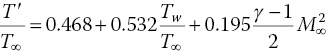
In particular, for both laminar and turbulent flows, the reference temperature (Tref), based on Eckert’s method, reads:
where the recovery factor, Rf, is calculated as the square root of the Prandtl number for laminar flows, and the cube root of the Prandtl number for turbulent flows. The Prandtl number is evaluated at the reference temperature.
For laminar flows, the skin friction coefficient and Stanton number are calculated as:

For turbulent flows the relations for skin friction and Stanton number are:

In the above relations, Mf is the Mangler factor. For laminar flows, Mf is equal to 3 and for turbulent flows it is set to 2. The enthalpy‐based film coefficient, recovery enthalpy and convective heating are defined as:
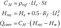
In the above relations, He is the edge static enthalpy, Hrec is the recovery enthalpy, Ue the edge velocity, and Hw is the wall enthalpy. Hw can be evaluated both at cold and radiative cooling wall boundary conditions. In the latter case, a Newton–Raphson technique is used to assess the wall temperature, with the energy radiated from the surface equal to the sum of the convective and incident shock‐radiative heatings:
Indeed, since the convective heating depends on the final wall temperature, this non‐linear relationship must be solved iteratively at each panel centroid.
With the leading‐edge boundary‐layer model, the vehicle nose and leading edge may be modelled as either a sphere, cylinder or a swept cylinder. For instance, the stagnation point convective heat transfer for spherical and unswept cylinder leading edges, according to Fay and Riddell, reads:

where the index k = 0 for 2D flow and k = 1 for axisymmetric flow. Here the subscripts w, e, and s denote conditions at the wall, the external flow, and the stagnation point. φ = 0.52 for the equilibrium boundary layer and φ = 0.63 for the frozen boundary layer and a fully catalytic wall.
The term in square brackets represents the effects of equilibrium chemical reactions occurring in the stagnation region and:

The Prandtl number Pr and the Lewis number Le are nondimensional parameters, like the Reynolds number, and measure the relative importance of friction to heat conduction and of species diffusion (mixing) to conduction, respectively. The gas considered is air, which, for the purposes of mixing, can be considered to be a binary mixture of two species: atoms (O or N) and molecules (O2 and N2). The quantity D12 is the binary diffusion coefficient that measures the ability of species 1 to mix with species 2. The quantities ci and Δhf,i are the molar concentrations of the individual species present (O, O2, N, and N2) and the chemical heat of formation of each of the species, respectively.
The Lewis number for air‐like mixtures is close to unity: Le~1.4, so that the quantity (Le0.52−1) ≈ 0.19, and the contribution of the chemical reaction term can often be safely neglected in preliminary studies.
The velocity gradient along the x‐axis – that is, along the body surface – at the stagnation point is:

Next, the methods used for spherical and unswept cylinder leading edges include Lee’s method for laminar flow and the Detra–Hildalgo method for turbulent flow. These provide heat flux distributions around the leading edge.
As far as the influence of leading edge sweep angle is concerned, the analysis uses Lee’s method with the addition of the sweep angle effect (Ksweep). According to the swept cylinder method, this reads:

where Ksweep, according to Cato–Johnson, is:
while for Beckwith–Gallagher it reads:
where Λ is the leading edge sweep angle.
The CFD code FLUENT solves the full Reynolds‐averaged Navier–Stokes (RANS) equations in a finite‐volume approach, with a cell‐centred formulation on a multi‐zone block‐structured grid. In the present research effort, the thermal and chemical non‐equilibrium flow field governing equations are integrated in a density‐based approach with a flux difference splitting second‐order upwind numerical scheme for the spatial reconstruction of the convective terms. For the diffusive fluxes, a cell‐centred scheme is applied. In some computations, however, the flux vector is computed by using a flux‐vector splitting scheme called the advection upstream splitting method. This provides an exact resolution of contact and shock discontinuities and it is less susceptible to carbuncle phenomena.
An implicit solver formulation was considered in the computations. Indeed, due to broader stability characteristics of the implicit formulation, a converged steady‐state solution can be obtained much faster using the implicit formulation rather than the explicit formulation.
Calculation of global transport properties of the gas mixture relied on semi‐empirical rules such as Wilke’s mixing rule for viscosity and thermal conductivity. The viscosity and thermal conductivity of the ith species was obtained from the kinetic theory of gases. For the diffusion coefficient of the ith species in the mixture, the multi‐component diffusion coefficient was applied, with species mass diffusivity evaluated by kinetic theory. Flowfield chemical reactions proceed with forward rates that are expressed in the Arrhenius form, while reaction‐rate parameters are due to Park [37]. In particular, a number of in‐house modifications (user defined functions; UDF) for the thermal non‐equilibrium were used, since vibrational non‐equilibrium conditions are not basic code features. In the UDF, vibrational relaxation is modelled using a Landau–Teller formulation, where relaxation times are obtained from Millikan and White, assuming simple harmonic oscillators.
Finally, the k‐ω SST model was used to account for turbulence effects and only steady state computations have been carried out so far.
3.9 Aerodynamic Characterization
Usually the vehicle aerodynamic characterization is provided in terms of force and moment coefficients, and control surfaces effectiveness. The force coefficients are lift (CL), drag (CD), and side (CY) and the moments refer to rolling (Cl = Cmx), pitching (Cm = Cmy), and yawing (Cn = Cmz) coefficients, according to the following equations.

where Sref is the reference surface (usually the vehicle planform area), Lref is the longitudinal reference length (usually the fuselage length, L), and bref is the lateral‐directional reference length (usually the wing‐span).
3.9.1 ORV Aerodynamic Reference Parameters
For the ORV concept the geometric reference parameters (see Figure 3.35) that have been chosen in order to make aerodynamic forces (FL, FD, and FY) and moments (Mx, My, and Mz) non‐dimensional coefficients are:
- Lref (mean aerodynamic chord)
- bref (wing span)
- Sref (wing area).
The pole coordinates are (xCoG/L,0,0) m.
Figure 3.35 Aerodynamic reference parameters.
3.9.2 Reference Coordinate System and Aerodynamic Sign Conventions
In Figure 3.36 the reference frames adopted are shown. The subscript b indicates the body reference frame (BRF), s refers to the stability reference frame (SRF); while w indicates the wind reference frame (WRF). The origin of both reference systems is in the CoG of vehicle. The pole for the calculation of the moment coefficients is assumed as the CoG; the positive x‐axis for the ORV body‐axis system is shown parallel to the fuselage reference line.
The aerodynamic reference axis systems are sets of conventional, right‐hand, orthogonal axes with the x‐ and z‐axes in the plane of symmetry and with the positive x‐axis directed out of the nose (in the body‐axis system) or pointing into the component of the wind (in the stability‐axis system) that lies in the plane of symmetry.

Figure 3.36 Reference frames.
The reference system for the aerodynamic data is a body‐fixed axis system, compliant with the ISO 1151 standard (see Figure 3.37, in which the aerodynamic coefficient convention and sign rules are also provided).
Figure 3.37 Reference frames and aerodynamic sign conventions.
Therefore, normal force (CN), axial force (CA), side force (CY), rolling moment (Cl), pitching moment (Cm), and yawing moment (Cn) coefficients refer to the BRF. Lift force (CL) and drag force (CD) coefficients are provided in the WRF.
The following aerodynamic sign convention (see Figure 3.37 where directions are positive as shown) for forces, moments, and velocity is adopted:
- AoA (α) is positive when free stream arrives from down of the pilot.
- Sideslip angle (β) is positive when free stream arrives from right of the pilot.
- Aileron deflection angle (δa) is positive when trailing edge is down.
- Elevon deflection angle (δe) is positive when trailing edge is down.
- Body flap deflection angle (δbf) is positive when trailing edge is down.
- Rudder deflection angle (δr) is positive when trailing edge turns on the left of the pilot.
- Axial force coefficient (CA) is positive when force is pushing in front of vehicle towards the base.
- Normal force coefficient (CN) is positive when force is pushing upwards on the belly side of vehicle.
- Side force coefficient (CY) is positive when force is pushing on the left‐hand side of the vehicle towards the right.
- Rolling moment coefficient (Cl) is positive when the right wing is down.
- Pitching moment coefficient (Cm) is positive when the aircraft is nose up.
- Yawing moment coefficient (Cn) is positive when the right wing is backward.
This is the convention usually adopted in flight mechanics. As a result, the static stability conditions for the vehicle are the following:
- longitudinal static stability: Cmα < 0
- lateral‐directional static stability: Cnβ > 0; Clβ < 0.
ORV aerodynamic control surface deflections, forces, and hinge moments are illustrated in Figure 3.38 and summarized in Table 3.4. In general, control surface deflection angles are measured in a plane perpendicular to the control surface hinge axis. An exception is the rudder control surface deflections, which are measured in a plane parallel to the fuselage reference plane.
Figure 3.38 ORV aerodynamic control surface deflections, forces, and hinge moments.
Table 3.4 ORV aerodynamic control surface deflections, forces, and hinge moments.
| Positive deflection of | Aero forces and moments |
| Rudder, δr | +CY, −Cn |
| Elevon, δe | −Cm |
| Right, δe,R | −Cl |
| Left, δe,L | +Cl |
3.9.3 Inputs for ORV AEDB Generation
Based on the re‐entry flight scenario in Figures 3.15 and 3.16 the aerodynamic data set has been generated for the flight envelope bounded by the ranges shown in Table 3.5.
Table 3.5 Flight envelope ranges.
| Parameter | Value | Comment |
| Subsonic to supersonic flow conditions | ||
| M∞ | [0.3, 0.5, 0.7, 0.9, 1.1, 1.3, 1.5, 1.7] | |
| Re∞/m | 1 × 10⁷ m−1 | |
| α | [0, 2, 4, 6, 8, 10, 12, 14, 16, 18, 20] | |
| β | [−8, −4, −2, 0, 2, 4, 8] | |
| δ | [−30, −20, −10, 10, 20, 30] | For aileron, elevon and rudder |
| For the remaining part of the re‐entry trajectory | ||
| M∞ | [2, 3, 4, 6, 8, 12, 16, 20, 25] | |
| Re∞/m | [2 × 10⁴, 105, 5 × 10⁵, 2 × 10⁶] | |
| α | [0, 2, 5, 7, 10, 12, 14, 15, 17, 20, 22, 25, 27, 30, 35, 40, 45, 50] | |
| β | [−4, −2, 0, 2, 4] | |
| δ | [−30, −20, −10, 10, 20, 30] | For aileron, elevon and rudder |
It must be noted that the range of Reynolds number was chosen to cover a wide part of the re‐entry, based on a preliminary re‐entry trajectory, as shown in Figure 3.39, which shows the ORV preliminary reference flight envelope, together with the iso‐Mach and iso‐Reynolds curves, in an altitude–velocity map.

Figure 3.39 ORV re‐entry scenario in an altitude–velocity map with iso‐Mach and Reynolds curves.
3.9.4 ORV Aerodynamic Model
This section contains the ORV aerodynamic model (AM) for the development of the vehicle AEDB, used for flight mechanics analysis, subsystem design and analyses, as well as for flight control analysis.
An important aspect of developing an AEDB is the formulation of an aerodynamic model. For example, the accuracy of the database depends on the degree to which the AM represents the physics of the problem. Therefore, it is important that all the aerodynamic and control variables that may have influences on the given aerodynamic coefficient be included in the aerodynamic model. To this end, a number of hypotheses have been assumed in developing the ORV AM. The independent variables that have been recognized as having influence on the ORV aerodynamic state are the set: ![]()
The couple (M, Re)4 identifies the aerodynamic environment, while the remaining variables completely describe the flowfield direction. Therefore, the functional structure of the AM of the ORV is based on these independent variables. Note, however, that the AEDB under development at this phase of the project does not consider the contribution of dynamic effects because low‐order methods, widely used in this framework, are unable to reliably determine this contribution.
As done in the past for the US Orbiter and X‐34 vehicles, the ORV AM development relies on the following assumptions:
- No RCS effects are considered.
- Only rigid body aerodynamic coefficients are evaluated; in other words, no aero‐elastic deformations are accounted for.
- No Reynolds and Knudsen numbers effects on aerodynamic control surfaces are assumed.
- No sideslip effects on aerodynamic control surfaces are assumed, except for rudder efficiency.
- No effects of protrusions, gaps and roughness are considered.
- No Knudsen numbers effects on side force and aerodynamic moment coefficients are assumed (except for pitching moment coefficient).
- No mutual aerodynamic interference between control surfaces is considered.
Finally, it is worth noting that, as typically done in a classical approach, each aerodynamic coefficient can be derived by supposing that each contribution to the single global coefficient is independent from the others. This means, from an operational point of view, that each aerodynamic coefficient is described by a linear summation over a number of incremental contributions (in other words, a build‐up approach). Each contribution is based on a small number of parameters.
3.9.5 Formulation of the Aerodynamic Database
The aerodynamic characteristics pertaining to the longitudinal (in other words, CL, CD, and Cm) and lateral (CY, Cl, and Cn) degrees of freedom are presented as full‐scale rigid force and moment coefficients. They are presented in a form that allows a build‐up to any desired configuration and/or flight condition by increments to the basic coefficient.
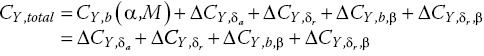
Each aerodynamic coefficient has been considered separately using the appropriate equation in which all the required contributions for obtaining the total coefficient for any selected flight condition appear. Following the formulation used for the Space Shuttle and assuming that the vehicle is operating at a combined AoA (α), and AoS (β), the total lift coefficient is given by:

where CL,total is the total lift coefficient of the vehicle for a given flight condition as expressed by the flight Mach number M, AoA is α, sideslip is β, elevon deflection is δe, ailerons deflections are δa, body flap deflections are δbf, and rudder deflection is δr. The parameter CL,b(α, M, Re) is the baseline lift coefficient at zero sideslip and zero control surface deflections (in other words, in a clean configuration). It also takes into account rarefaction effects through a bridging relationship. The parameter ![]() represents the incremental lift coefficient due to elevon deflections above the baseline and is given by:
represents the incremental lift coefficient due to elevon deflections above the baseline and is given by:
The parameter ΔCL,δa represents the incremental lift coefficient due to aileron deflections above the baseline and can be evaluated using the data on elevons as follows:

Here, we use the elevon data twice; once assuming δe = δe,L, obtaining ![]() and then assuming δe = δe,R to determine
and then assuming δe = δe,R to determine ![]() . As a check, when the aileron deflection is zero, in other words, δe = δe,L = δe,R, the value of
. As a check, when the aileron deflection is zero, in other words, δe = δe,L = δe,R, the value of ![]() vanishes as expected.
vanishes as expected.
The parameter ![]() represents the incremental lift coefficient due to body flap deflections above the baseline and is given by:
represents the incremental lift coefficient due to body flap deflections above the baseline and is given by:
The incremental lift coefficient ![]() due to the rudder is defined as follows:
due to the rudder is defined as follows:
The incremental lift coefficients due to the baseline and rudder in sideslip are given by:
Note that the first term in square brackets on the right‐hand side of the last equation gives the combined incremental coefficient due to the rudder at an AoA and sideslip over the baseline at the same values of AoA and AoS. To get the incremental coefficient due only to sideslip β, we have to subtract the incremental due to AoA as shown by second term on the right‐hand side of equation.
Those contributions represent aerodynamic cross‐coupling effects, and they have been found to be significant, especially at higher values of AoA.
In a similar fashion, we assume that the drag and pitching moment coefficients are given by:


The change in pitching moment coefficient due to rudder deflection, ![]() , is assumed to be zero. The side force coefficient is assumed to be given by:
, is assumed to be zero. The side force coefficient is assumed to be given by:
since the vehicle configuration is symmetric; in other words, ![]() . Furthermore,
. Furthermore,
Similarly,

Then,
where the incremental side force coefficient due to rudder is sideslip is defined as
Proceeding in a similar way, the rolling and yawing moment coefficients are assumed to be given by:
Therefore, it is assumed that the sideslip has effect only on the baseline, and when the rudder is deflected, but it has no effect when the elevons, body‐flap or ailerons are deflected.
Moreover, as stated above, no dependency on Reynolds number is assumed for the elevon contribution. Indeed, even though this effect exists it is small and difficult to model. It has been considered as part of the uncertainty of the aerodynamic coefficients.
3.9.6 Process of Development of the Aerodynamic Database
The above formulation of the AM for free flight provides a framework for building the ORV AEDB. It consists of aerodynamic data tables in the form of total and incremental coefficients. These are provided in a convenient form so that the user can evaluate each of the terms in the free‐flight aerodynamic models, and then sum them to get the desired aerodynamic coefficient.
In particular, the ORV AEDB relies on following segments:
- the free‐molecular flow conditions
- the transitional flow conditions
- the continuum flow conditions
- hypersonic flow
- supersonic flow
- transonic flow
- subsonic flow.
Figure 3.40 is a guideline used in developing vehicle AEDBs.
Figure 3.40 ORV flow regime in the altitude‐Mach map.
It shows the ORV reference flight scenario in an altitude‐Mach map together with the altitude limits that bound the different flow regimes.
Finally, it is worth noting that in transitional flow conditions a very simple relationship to bridge the FMF regime to continuum flow (see Figure 3.40) can be given as:
where the normalized coefficient ![]() uses the Knudsen number as the independent parameter:
uses the Knudsen number as the independent parameter:

where 10−3<Kn∞<10 and CiContinuum and CiFM are the aerodynamic coefficients in the continuum and FMF regimes, respectively. This formula was used for the US Orbiter aerodynamics assessment [31].
The results of each AEDB segment are described in detail in the next sections.
3.10 Low‐order Methods Aerodynamic Results
Simplified aerodynamic analyses for supersonic and hypersonic speeds were performed on panel meshes similar to those shown in Figure 3.41.

Figure 3.41 Examples of the ORV panel mesh.
3.10.1 HPM Results for Rarefied and Transitional Flow Conditions
As shown in Figures 3.17 and 3.40, above 200 km altitude the ORV experiences FMF conditions. This means that particle simulations, such as DSMC, should be performed to address the vehicle aerodynamics. At an early design stage, however, only low‐order analyses, such as those obtained from SIM computations, can be carried out. The aerodynamic analysis was performed on the vehicle in a clean configuration, and at a free‐stream velocity of 7330 m/s, considered constant with altitude. In all computations the wall temperature was set equal to 300K (with a body temperature ratio equal to 0.351), and the aerodynamic forces were evaluated on the assumption of a fully accommodated Maxwell model. Free‐stream thermodynamic parameters were provided by the US Standard Atmosphere, 1976.
The ORV aerodynamics in FMF conditions are summarized in Figures 3.42–3.44.

Figure 3.42 ORV‐WBB lift coefficient vs AoA in FMF.


Figure 3.44 ORV‐WBB aerodynamic efficiency vs AoA in FMF.
These figures highlight that FMF conditions result in an abrupt loss of vehicle aerodynamic efficiency due to a sudden increase in drag and lift drop.
As far as transitional‐flow aerodynamics are concerned, Figures 3.17 and 3.40 show that the ORV flies in that regime from about 200–87 km altitude. Lift, drag and pitching moment coefficients versus the Knudsen (KnLref∞) number are reported in Figures 3.45–3.48 for AoAs of 10, 20, 30, and 40°. The behaviour of the lift coefficient at 10 and 20° and at 30 and 40° is shown in Figures 3.45 and 3.46, respectively.

Figure 3.45 Lift coefficient vs Knudsen number for ORV‐WBB at AoA = 10 and 20°.

Figure 3.46 Lift coefficient vs Knudsen number for ORV‐WBB at AoA = 30 and 40 deg.
The variation of drag and pitching moment coefficient of ORV‐WBB at 30 and 40° AoA, along with the Knudsen number is reported in Figures 3.47 and 3.48, respectively.

Figure 3.47 Drag coefficient vs Knudsen number for ORV‐WBB at AoA = 30 and 40°.

Figure 3.48 Pitching moment coefficient vs Knudsen number for ORV‐WBB at AoA = 30 and 40°.
The classical S‐shape of the bridging formula is clearly recognized, ranging from continuum to FMF. Furthermore, note that in each figure the variation of the altitude with Knudsen number is also provided to help the reader understand with what flight conditions the aerodynamic results must be associated. The effect of rarefaction on the aerodynamic lift results in an abrupt loss of CL. For example, at AoA = 40° CL decreases by about 87.5% from 80 km to 200 km. The same consideration applies for Cm. As far as aerodynamic drag is concerned, Figure 3.47 shows that CD at AoA = 30° increases by about 200% from 90 km to 110 km, whereas the drag at H = 200 km is 250% higher than at 90 km. Therefore, the strong reduction of the aerodynamic efficiency due to rarefaction effects is very clear in Figure 3.49.

Figure 3.49 ORV‐WBB aerodynamic efficiency vs Knudsen number for AoA = 30 and 40°.
3.10.2 HPM Results for Continuum Flow Condition
HPM results refer to both clean and flapped configurations. Trade‐off design analyses highlight that the best surface inclination methods (see Table 3.3) to consider in assessing vehicle aerodynamic performance in continuum flow conditions are the empirical tangent cone and tangent wedge, for the fuselage5 and wing windside, respectively. A modified Newton–Prandtl–Meyer approach is used for the leading edges and the Newtonian method (in other words, cp = 0) applies at the vehicle leeside [32, 33].
Some of main results obtained for the ORV‐WSB for clean‐configuration aerodynamics (in other words, no aerodynamic surfaces deflected) are shown in Figures 3.50–3.53.

Figure 3.50 ORV‐WSB aerodynamic polars for 2≤M∞≤9.

Figure 3.51 ORV‐WSB aerodynamic polars for M∞ = 10, 16, and 25.

Figure 3.52 ORV‐WSB pitching moment coefficient for M∞ = 2, 3, 6, and 9.

Figure 3.53 ORV‐WSB pitching moment coefficient for M∞ = 10, 15, 20, and 25.
Figures 3.50 and 3.51 show the aerodynamic polars and Figures 3.52 and 3.53 the pitching moment coefficients for Mach numbers ranging from 2 to 25 and α from 0 to 40°. As shown, ORV‐WSB drag and lift decrease as Mach number increases, ultimately reaching a value that does not change even if Mach still rises, according to the Oswatich principle (in other words, independence of aerodynamic coefficients from M∞) starting from M∞ = 10 [13, 17]. Figure 3.52 also shows that at M∞ = 2 and M∞ = 3 the pitching moment derivative is negative for α larger than 5° and 15°, respectively. At hypersonic conditions, the configuration is statically stable (in other words, Cmα < 0) for α higher than 20°. In particular, the concept in clean configuration features a natural trim point (Cm = 0) at about 33–38° AoA for M∞ = 6 and 9. At higher Mach number trims, AoA ranges from about 42 to 44° (see Figure 3.53).
As far as the lateral‐directional stability is concerned, Figure 3.63 shows for α = 5° the effect of sideslip on the rolling (Cl) and yawing moment (Cn) coefficients, along with Mach number.

Figure 3.63 ORV‐WSB: effect of sideslip on Clβ and C nβ up to M∞ = 9, at α = 5°.
As shown, the configuration is statically stable in lateral‐directional flight at α = 5°. Note that the body flap is advantageous for both longitudinal and lateral‐directional stability by providing margins on the CoG location. In fact, the body flap, located on the rear lower portion of the aft fuselage, allows the vehicle to be pitch trimmed, while the elevons provide roll control. The lift‐to‐drag ratio of ORV‐WSB and ORV‐SB concepts is shown in Figure 3.64 for Mach numbers ranging from 2 to 9 at α = 5°.

Figure 3.64 L/D versus Mach at α = 5°. Comparison between ORV‐WSB and ORV‐SB concepts.
The ORV‐SB concept has enhanced aerodynamic efficiency due to its highly streamlined aeroshape compared with ORV‐WSB, as expected.
Figure 3.65 shows the aerodynamic lift coefficients for ORV‐WSB, ORV‐WBB and ORV‐SB. ORV‐SB and ORV‐WBB feature the same lift slope, which is larger than that of ORV‐WSB.

Figure 3.65 Lift coefficients at Mach 10 for ORV‐WSB, ORV‐WBB and ORV‐SB.
The comparison of aerodynamic drag is shown in Figure 3.66. In this case, and in that of lift, discussed above, differences in aerodynamic performance at low AoAs are dictated by differences in fuselage forebody slopes and cross‐sectional areas (see Figure 3.11). Indeed, the larger the vehicle’s cross‐section the greater the drag coefficient.
On the other hand, at high AoAs, differences in aerodynamic coefficients are due to the different planform shapes that characterize each concept (see Figure 3.11). The ORV‐WSB has the lower planform surface.

Figure 3.66 Drag coefficients at Mach 10 for ORV‐WSB, ORV‐WBB and ORV‐SB.
The slope of the lift and drag coefficients is close respectively to sin2α•cosα and sin3α, as stated by impact flow theory [13, 17, 34, 35].

Figure 3.67 Lift‐to‐drag ratio at Mach 10 for ORV‐WSB, ORV‐WBB and ORV‐SB.
Differences in aeroshape, discussed above, result in different L/D profiles6 versus AoA, of course. For instance, L/D sharply increases with α in the case of streamlined configurations, but (L/D)max decreases as vehicle bluntness increases (the larger the vehicle bluntness the lower the peak aerodynamic efficiency) see Figure 3.67. It is worth noting that this high (L/D) slope of very streamlined aeroshapes is extremely important for scramjet‐propelled vehicles, since this kind of spacecraft must fly at small AoAs in order to assure proper airflow conditions at the scramjet intake and to minimize aerodynamic drag. In particular, the ORV‐SB concept features the best lift‐to‐drag ratio of the three concepts up to about α = 20° and it has an (L/D)max equal to about 2.8 at α = 10°. On the other hand, the maximum aerodynamic efficiency of ORV‐WB and ORV‐WBB is reached at about α = 15° at about 2.4 and 1.5, respectively.
For AoAs larger than 20°, differences in aerodynamic efficiency decrease as α increases, and they vanish for α > 35°. As a result, in the framework of re‐entry at high AoAs (35–40°; close to the AoA of the US Orbiter), differences in aeroshape do not significantly affect the descent flight. In fact, as said before, at hypersonic speeds and at high AoAs, vehicle aerodynamics are dictated essentially by planform shapes.
As far as the pitching moment is concerned, the effect of the CoG position (with respect to the fuselage length) on the Cm for each vehicle concept is summarized in Figure 3.68. When the CoG is at 63% of the fuselage length, ORV‐SB features a strong static instability in longitudinal flight, highlighting that the centre of pressure is well ahead of the CoG (in other words, there is a negative static margin); ORV‐WBB is static stable in pitch for α > 40° and can be trimmed by positive flap deflections; ORV‐WSB is static stable in pitch for α > 30° and also has a natural trim point at about 45° AoA.

Figure 3.68 Effect of CoG position on Cm at Mach 10 for ORV‐WSB, ORV‐WBB and ORV‐SB.
However, for a CoG at 56% of the fuselage length, the ORV‐SB concept becomes statically stable in longitudinal flight for α > 35° and trim AoA can be attained by positive flap deflections; the other two concepts (WSB and WBB) are statically stable in pitch for α > 5° and feature a natural trim point at 10 and 20° AoA, respectively. In particular, they can be trimmed at high AoA by means of negative (in other words, trailing‐edge up) flap deflections.
Note that, in statically stable and trimmed flight the attitude of the vehicle is aligned in such a way that the total external moment acting on the vehicle is zero. This means that after a disturbance the vehicle tends always to move back towards the trimmed state.
Pitching moment behaviour versus AoA indicates that vehicle subsystem arrangements (in other words, CoG position) must be carefully addressed. Indeed, in order to have a static stable and trimmable vehicle concept, the CoG has to be carefully chosen with reference to the vehicle shape.
3.11 CFD‐based Aerodynamic Results
For the numerical flowfield computations, on the basis of the flight envelope of Figure 3.15 a number of flight conditions have been chosen for CFD computations in steady‐state conditions, according to the space‐based design approach [13, 17, 34,35,36].
Numerical results aim to anchor engineering analyses in order to increase their accuracy, and to focus on some critical design aspects that are not predictable with simplified tools, for example SSI and shock‐wave–boundary‐layer interactions (SWIBLI) and high‐temperature real‐gas effects. SSI determines pressure and heat flux overshoots on the leading edges of both wing and tail, which must be accounted for in TPS design; SWBLI influences control surface effectiveness. The CFD test matrix is shown in Table 3.6.
Table 3.6 CFD test matrix.
| CFD test matrix | ||||||||||
| AoA @ AoS=0 deg | AoS @ AoA=5 deg | |||||||||
| Mach | 0 | 5 | 10 | 20 | 30 | 40 | 45 | 2 | 4 | 8 |
| 0.3 | X | X | X | X | ||||||
| 0.5 | X | X | X | X | ||||||
| 0.8 | X | X | X | X | ||||||
| 0.95 | X | X | X | X | ||||||
| 1.1 | X | X | X | X | ||||||
| 1.25 | X | X | X | X | ||||||
| 2 | X | X | X | X | X | |||||
| 3 | X | X | X | X | X | X | X | |||
| 4 | X | X | ||||||||
| 5 | X | X | X | X | X | |||||
| 6 | X | X | X | X | ||||||
| 7 | X | X | X | X | ||||||
| 8 | X | X | ||||||||
| 8 | Y | Y | ||||||||
| 10 | Y | Y | Y | |||||||
| 16 | Y | Y | Y | |||||||
| 20 | X | X | X | X | ||||||
| 20 | X | X | X | X | ||||||
| 25 | Y | Y | ||||||||
X, perfect gas; Y, reacting gas. Note that each cell identifies a CFD run (in other words, check point).
It is worth nothing that at M∞ = 8, 10, 16, and 20, non‐equilibrium CFD computations are also carried out. Real‐gas effects can be important because, during atmospheric re‐entry, dissociation processes take place in the shock layer, which can have an influence on the aerodynamic coefficients. High‐temperature real‐gas effects are expected to influence stability and control derivatives of the vehicle, in particular its pitching moment, as highlighted by the first Space Shuttle re‐entry (STS‐1), where an nose‐up pitching moment required a body‐flap deflection twice than that predicted by the pre‐flight analyses in order to trim the vehicle [36].
Furthermore, real‐gas effects cause a shock closer to the vehicle than a perfect gas theoretically would (in other words, there is a thin shock layer) [35,36,37]. This means that a strong SSI phenomenon arises. These effects obviously occur only at high Mach numbers [37].
Numerical non‐equilibrium investigations allow assessment and characterization of the wall catalyticity in order to reduce the design margins, preventing use of the overly conservative hypothesis of a fully catalytic wall, as usually used in TPS design.
CFD simulations also help in finding the effect of laminar‐to‐turbulent transitions, which must be accounte for in vehicle TPS design. It is well known that these transiations can cause strong and even dangerous overheating of the vehicle skin [38,39,40].
Numerical CFD computations have been carried out on both multi‐block structured and hybrid unstructured grids, similar to those shown in Figures 3.69 and 3.70. Figure 3.69 shows the sub‐transonic computational domain that were considered when addressing ORV‐WSB aerodynamics at sub‐transonic speeds.

Figure 3.69 Sub‐transonic computational domain: mesh on symmetry plane and ORV‐WSB surface.
The external boundary of the half‐body grid has been built as a Cartesian block, and far‐field surfaces are located at about ten body lengths away from the body (upstream and downstream) to ensure that the flow at the boundary is close to free stream. Indeed, the farther we are from the vehicle, the less effect it has on the flow and so the more accurate is the farfield boundary condition.
Close‐up views of the 3D sup‐hypersonic mesh on both the vehicle surface and the symmetry plane can be seen in Figure 3.70 for ORV‐WSB (left) and ORV‐WBB (right).
Figure 3.70 Sup‐hypersonic computational domain: mesh on symmetry plane and vehicle surface.
Of course, for all the computational domains, made of about 6 × 10⁶ cells (half body), the distribution of surface grid points is dictated by the level of resolution desired in various areas of vehicles, such as the stagnation region. Grid refinements in strong gradient regions of the flowfield are addressed by means of a solution‐adaptive approach. The coordinate y+ of the first cell adjacent to the surface is about 1.
As far as numerical results are concerned, it is worth noting that they refer to both converged and grid‐independent computations. Figures 3.71 and 3.72 show the ORV‐WSB aerodynamics at Re = 106, for Mach numbers ranging from 0.3 to 5 and for α = 0, 5, 10, and 20°. As shown, lift and drag coefficients rise in the transonic region, where the presence of the shock wave produces a large increase of the aerodynamic forces on the vehicle: the increase of wave drag and base drag that in this region reach their maximum values, as expected. On the other hand, when Mach number increases, aerodynamic coefficients tend to reach a limit value, according to the Mach number independence principle (the Oswatich principle).
In particular, this behaviour is similar for all the considered AoAs, and the strong dependence of the drag on the AoA is essentially due to the large increases of the induced drag with α [41,42,43,44].
Figure 3.71 Lift coefficient versus Mach number for different AoAs; ORV‐WSB concept.

Figure 3.72 Drag coefficient versus Mach number for different AoAs; ORV‐WSB concept.
Figure 3.73 shows the aerodynamic lift, drag and L/D versus α at M∞ = 0.3. Aerodynamic results at these flight conditions are extremely important considering that M∞ = 0.3 represents the nominal landing condition at the end of an unpowered re‐entry flight. Figure 3.73 shows that the lift coefficient at M∞ = 0.3 steadily increases from α = 0 to 20° indicating that the vehicle does not stall up to 20° at this Mach number. Therefore, the drag coefficient at zero AoA is about 0.047 and it continues to rise as AoA increases, and is expected to reach about 0.22 at α = 20°. The maximum L/D, close to 3.5, is attained at α = 10°. Of course, extra lift can be provided by means of positive flap deflections, thus also providing static stable trim conditions at landing AoA.
Figure 3.73 C L, CD and L/D versus AoA for M∞ = 0.3; ORV‐WSB concept.

Figure 3.74 Drag polars for 0.3 ≤ M∞ ≤ 1.25 and for α = 0, 5, 10, and 20°; ORV‐WSB concept.
In Figure 3.74 vehicle polars for Mach numbers ranging from 0.3 to 1.25 and for α = 0, 5, 10, and 20° are also reported, thus showing ORV‐WSB’s aerodynamics in sub‐transonic flow conditions.
The variation of the pitching moment coefficient of ORV‐WSB versus α is presented in Figure 3.75.

Figure 3.75 C m vs α at different Mach numbers. ORV‐WSB concept.
At low subsonic speeds (Mach 0.3 and 0.8), the ORV‐WSB vehicle is statically unstable in longitudinal flight (in other words, Cmα > 0) with the given CoG for all the considered AoAs. Concept stability changes for Mach numbers larger than 0.95. This means that at these flight conditions a perturbation that produces an increased angle of attack causes a nose‐down (negative) pitching moment, which decreases the AoA, restoring the vehicle to its original position. In particular, Cm in the sub‐transonic regime follows a fairly linear trend. Furthermore, the AoA at which the moment coefficient about the centre of gravity equals zero (in other words, trim condition) is approximately 5° for M∞ = 0.30 and M∞ = 0.95, 12° at M∞ = 0.80, and α = 2° for M∞ = 1.25.
In order to demonstrate the subsonic aerodynamic performance, Figures 3.76–3.78 show the pressure coefficient contour maps over the ORV‐WSB surface for all the analyzed AoAs at M∞ = 0.3.

Figure 3.76 Pressure coefficients at M∞ = 0.3 and for α = 0 and 5°; ORV‐WSB concept.
On the leading edge, we see a stagnation point where the velocity of the flow is nearly zero. The fluid accelerates on the upper surface (in other words, leeside) as highlighted by the negative value of Cp (in other words, pressure less than that of the surrounding atmosphere). On the other hand, at the trailing edge, the flow on the upper surface decelerates and converges with the flow on the lower surface (in other words, windside) according to the Bernoulli equation (in other words, whenever there are high velocities, we have low pressures and vice versa).
With the pressure distributions as sketched, the effect on the upper surface is the larger, and there is a resultant upwards force on the section, that is, lift.

Figure 3.77 Pressure coefficients at M∞ = 0.3 and for α = 10 and 20°; ORV‐WSB concept.
In particular, the pressure reduction on the upper surface increases both in intensity and extent at high incidence (see Figures 3.77 and 3.78); the stagnation point moves progressively further back on the lower surface, and the increased pressure on the lower surface covers a greater proportion of the surface, as shown in Figure 3.78.

Figure 3.78 Pressure coefficient at M∞ = 0.3 and for 0≤α≤20°; ORV‐WSB concept.
Therefore, the following conclusions may be drawn: at low incidence the lift is generated by the difference between the pressure reductions on the upper and lower surfaces; at higher incidences the lift is partly due to pressure reductions on the upper surface and partly due to pressure increases on the lower surface. Figure 3.79 shows the effect of AoA on the flowfield streamlines in the vehicle symmetry plane at M∞ = 0.3 and for α ranging from 0 to 20°. Streamtraces are displayed in order to highlight the flowfield structure surrounding the vehicle, especially the complexity of the wake flow. There is a rather strong base expansion together with a vortex feature. Indeed, for all the AoAs, a pattern of two swirling vortices is clearly visible in the wake flow. This kind of pattern is close to those known as von Karman vortices. These swirling vortices characterize the unsteady7 downstream separation of flow over the blunt bodies (in this case the vehicle base). This brings about an increase in drag (in other words, pressure drag). It is worth noting that space vehicles need drag to decelerate during the atmospheric descent, in order to lose as much internal energy (kinetic plus potential) as possible so that they can land safely. Therefore, space vehicles typically have a truncated afterbody (or blunt base), which results in base drag being a significant component of the total vehicle drag.

Figure 3.79 Pressure field past ORV‐WB, with streamtraces on the vehicle symmetry plane at M∞ = 0.3 and for α = 0, 5, 10 and 20°.
The blunt base of the re‐entry vehicle is also needed to allocate the nozzles of the rocket motor (as in the Space Shuttle Orbiter) for the boost needed in the ascent phase and the de‐boost necessary to start the de‐orbiting manoeuvre before atmospheric re‐entry (see nozzle at the base of ORV‐WBB in Figure 3.5).
In Figure 3.80 an example of the 3D flowfield streamtraces predicted by CFD computations is reported for the ORV‐WSB concept. It is possible to see the formation of the leading‐edge vortex, typical of delta‐wing configurations, and its interaction with the wing‐tip vortex.
Note that leading‐edge vortex lift is an important source of vehicle lift. The pressure on the upper surface of the wing is lower than that of the surrounding atmosphere, while the pressure on the windside is greater than that on the leeside. Thus, over the upper surface, air will tend to flow inwards towards the root from the tips, being replaced by air that was originally outboard of the tips. Similarly, on the undersurface, air will either tend to flow inwards to a lesser extent, or may tend to flow outwards. Where these two streams combine at the trailing edge, the difference in spanwise velocity will cause the air to roll up into a number of small streamwise vortices, distributed along the whole span. These small vortices roll up into two large vortices just inboard of the wing tips.

Figure 3.80 C p on ORV‐WSB surface with flowfield streamtraces at α = 20° and M∞ = 0.3.
In the following figures, some of main interesting hypervelocity flowfield features obtained for the ORV‐WSB concept are shown. For example, the Mach number and flow species fields for M∞ = 10 and 20 at AoA = 10, 30, and 40° are reported from Figures 3.81–3.85. Looking at the contour fields on the vehicle symmetry plane, one can appreciate the rather strong bow shock that occurs ahead of the vehicle concept during descent at these flight conditions, especially at higher AoAs. Figures 3.81 and 3.82 show the Mach number field past the rather sharp WBV for M∞ = 10 and for 10 and 30° AoA, respectively.

Figure 3.81 Mach contours on symmetry plane and ORV‐WSB surface at M∞ = 10 and α = 10°.
Figure 3.82 Mach contours on symmetry plane and ORV‐WSB surface at M∞ = 10 and α = 30°.
Figure 3.83 shows a blow‐up of the flowfield past the vehicle for both free‐stream conditions. Stream traces are also displayed.
Figure 3.83 Mach number contours on symmetry plane and vehicle surface at M∞ = 10 and α = 10 and 30°.
As shown, even if the CFD computations are carried out for perfect gas flow, the bow shock is very close to the vehicle because of its streamlined configuration.
The effect of AoA on the flowfield past ORV‐WSB flying at M∞ = 10 can be appreciated as well. Figure 3.84 displays a blow‐up of the flowfield surrounding the rather sharp wing body vehicle for M∞ = 20 and α = 40°. The Mach number and the static temperature contour field both on the vehicle symmetry plane and the concept outer surface are provided. Streamtraces are also displayed in order to highlight the flowfield structure surrounding the vehicle, especially the complexity of the wake flow. The flow stagnates downstream, thus increasing the local temperature distribution and a strong base expansion together with a vortex feature can be seen at α = 40°.

Figure 3.84 Non‐equilibrium CFD computation at H∞ = 70 km, M∞ = 20 and α = 40°. Mach and temperature contour fields; ORV‐WSB.
In this case, air was considered to be made up of five chemical species (O2, N2, O, N and NO) and in thermochemical non‐equilibrium conditions. The corresponding oxygen (O) and nitrogen oxide (NO) mass fraction contour fields are shown in Figure 3.85.
Figure 3.85 O and NO mass fractions. CFD computation at H∞ = 70 km, M∞ = 20 and α = 40°; ORV‐WSB concept.
As far as the AoS effect is concerned, Figure 3.86 shows the Mach number contours on a fuselage cross plane and those of the static pressure on the vehicle surface at M∞ = 6, α = 5° and β = 2°. Figure 3.87 shows the same flowfield features as Figure 3.86 but for M∞ = 3, α = 5° and β = 4 and 8°.

Figure 3.86 Mach contours on a fuselage cross plane and pressure contours on the vehicle surface at M∞ = 6, α = 5° and β = 2°. Euler computation for ORV‐WSB concept.

Figure 3.87 Mach contours on a fuselage cross plane and pressure contours on the vehicle surface at M∞ = 3, α = 5° and β = 4 and 8°. Euler computation for ORV‐WSB concept.
A different line of sight for M∞ = 3, α = 5° and β = 8° is provided in Figure 3.88.

Figure 3.88 Mach contours on two fuselage cross planes and pressure contours on the vehicle surface at M∞ = 3, α = 5° and β = 8°. Euler computation for ORV‐WSB concept.
The effect of sideslip angle on flowfield features is clearly shown in the non‐symmetrical distribution of the contour fields. This determines, apart from lift, drag and pitching moment, the lateral‐directional aerodynamic forces and moments acting on the vehicle concept.
Finally, Figures 3.89 and 3.90 show the pressure spike due to SSI that takes place on the ORV‐WSB at M∞ = 6, M∞ = 7 and α = 5°, respectively. Of course, the point of the wing leading edge where this interaction takes place depends on the free‐stream conditions.

Figure 3.89 Pressure coefficient distribution on the ORV‐WSB surface at M∞ = 6 and α = 5°.
Figure 3.89 shows the contour plot of the pressure coefficient on the vehicle surface and Figure 3.90 displays the Mach number on the wing plane. The pressure overshoot where SSI impinges the wing leading edge is clearly seen, as is the trace of the bow shock on the wing plane.
Figure 3.90 Pressure and Mach number distributions on ORV‐WSB surface and wing plane at M∞ = 7 and α = 5°.
Numerical flowfield results for the ORV‐WBB concept are shown in Figures 3.91 and 3.92 for M∞ = 25 and α = 30°. Figure 3.91 highlights the Mach number and the N2 mass fraction contour fields on the vehicle symmetry plane and cp on the concept outer surface.
Side and bottom views of the surface distribution of cp at these flight conditions are shown in Figure 3.92. Here, three flowfield cross‐sections are also shown to give an idea of the 3D bow shock that envelops the ORV‐WBB.

Figure 3.91 Mach (top) and N2 (bottom) contours on the symmetry plane and cp on the vehicle surface at M∞ = 25 and α = 30°; ORV‐WBB concept.

Figure 3.92 c p on vehicle surface at M∞ = 25 and α = 30°; ORV‐WBB concept.
Regarding the flowfield past the ORV‐SB concept, Figure 3.93 shows the Mach number contour field in the vehicle symmetry plane and the pressure distribution on the concept surface at M∞ = 25 and α = 30°. Streamlines are also provided.
Figure 3.93 c p on the ORV‐SB surface at M∞ = 25 and α = 30°.
3D streamtraces at these flight conditions together with a cross‐flow section coloured by Mach number are provided in Figure 3.94. A very narrow shock layer is also expected for this concept.

Figure 3.94 c p on the ORV‐SB surface at M∞ = 25 and α = 30° with 3D streamtraces and flowfield cross‐section coloured by Mach number.
To compare the aerodynamic results of numerical and engineering analyses, results for M∞ = 10, 20 and for 0 < α < 40° are provided in Figures 3.95 and 3.96 for the ORV‐WSB concept.
Figure 3.95 C L vs α; HPM and CFD results comparison at M∞ = 10 and 20; ORV‐WSB concept.

Figure 3.96 C D vs α; HPM and CFD results comparison at M∞ = 10 and 20; ORV‐WSB concept.
This confirms that engineering‐based (in other words, HPM) and numerical data match very well. Moreover, the differences between real‐gas and frozen‐gas coefficients, shown in Table 3.6 for M∞ = 20 and 10<α<40°., suggest that high‐temperature gas effects are negligible for lift and drag; whereas a significant effect on vehicle pitching moment is expected along the re‐entry trajectory varying from 8 to 50%.
Table 3.6 Real‐gas effects on ORV‐WSB aerodynamics.
| CL | |||
|
AoA (°) |
PG | RG | Error (%) |
| 10 | 0.1386 | 0.1402 | –1.15 |
| 20 | 0.4875 | 0.4809 | 1.37 |
| 30 | 0.9310 | 0.9130 | 1.97 |
| 40 | 1.3270 | 1.3079 | 1.46 |
| CD | |||
|
AoA (°) |
PG | RG | Error (%) |
| 10 | 0.0633 | 0.0610 | 3.80 |
| 20 | 0.2228 | 0.2185 | 2.00 |
| 30 | 0.5917 | 0.5817 | 1.72 |
| 40 | 1.1755 | 1.1645 | 0.94 |
| CM | |||
|
AoA (°) |
PG | RG | Error (%) |
| 10 | 0.0358 | 0.0432 | –17.01 |
| 20 | 0.0864 | 0.0939 | –7.98 |
| 30 | 0.0818 | 0.0958 | –14.55 |
| 40 | 0.0248 | 0.0476 | –47.82 |
Finally, numerical and engineering‐based aerodynamic results for ORV‐WBB and ORV‐SB are shown in Figures 3.97 and 3.98, respectively.

Figure 3.97 C A and CM at M∞ = 25 and α = 30°; CFD and HPM comparison; ORV‐WBB concept.

Figure 3.98 CA and CN at M∞ = 25 and α = 30°; CFD and HPM comparison; ORV‐SB concept.
Figure 3.97 compares the aerodynamic results for the axial force coefficient (CA) and pitching moment coefficient (CM) at M∞ = 25 and α = 30° (pole at vehicle nose); Figure 3.98 compares the results for the normal force coefficient (CN) at M∞ = 10 and α = 30° and for the axial force coefficient (CA) at M∞ = 25 and α = 30 and 45°. Here too, HPM provides reliable results in the framework of a phase‐A design.
References
- 1 The Atmospheric Reentry Demonstrator. ESA Bulletin. BR‐138, October 1998
- 2 P. Tran, J.C. Paulat, P. Boukhobza, ‘Re‐entry flight experiments lessons learned – the atmospheric reentry demonstrator ARD’. Technical report RTO‐EN‐AVT‐130, NATO RTO.
- 3 A. Schettino, R. Votta, P. Roncioni, et al. ‘Aerodynamic and Aerothermodynamic database of expert capsule’. Proceedings of the West‐East High Speed Flow Field Conference; 19–22 Nov 2007, Moscow, Russia.
- 4 S. Paris, D. Charbonnier, D. Tran, ‘Experimental and numerical investigation of aerothermal characteristics of the IXV hypersonic vehicle’. Paper presented at the 7th European Symposium on Aerothermodynamics for Space Vehicles. 9–12 May 2011, Brugge.
- 5 G. Pezzella, G. Marino, G. Rufolo, ‘Aerodynamic database development of the ESA intermediate experimental vehicle’. Acta Astronautica 2014, Volume 94, Issue 1, pp. 57–72.
- 6 A. Viviani, G. Pezzella, ‘Aerodynamic performance analysis of an unmanned re‐entry vehicle from hypersonic down to subsonic regime’. Proceedings of the 63rd International Astronautical Congress 2012, Naples, Italy.
- 7 A. Viviani, G. Pezzella, ‘Aerodynamic performance analysis of three different vehicle concepts at hypersonic speed’, Proceedings of the XXII Conference of Italian Association of Aeronautics and Astronautics, 9–12 Sept 2013. Naples, Italy.
- 8 ‘Aerodynamic problems of hypersonic vehicles.’ AGARD Lecture Series No. 42; Volume 1, Advisory Group for Aerospace Research and Development, 1997.
- 9 J.D. Anderson, Fundamental of Aerodynamics, McGraw‐Hill, 2001.
- 10 A. Schettino, G. Pezzella, et al., ‘Mission trade‐off analysis of the Italian USV reentry flying test bed’. Proceedings of the 14th AIAA‐AHI Space Planes and Hypersonic Systems and Technologies Conference; 6–9 Nov 2006, Canberra. Paper AIAA‐2006‐8017.
- 11 A. Schettino, G. Pezzella, et al., ‘Aero‐thermal trade‐off analysis of the Italian USV Re‐entry flying test bed’, Proceedings of the 14th AIAA‐AHI Space Planes and Hypersonic Systems and Technologies Conference; 6–9 Nov 2006, Canberra. Paper AIAA‐2006‐8114.
- 12 G. Pezzella, F. Battista, A. Schettino, et al., Hypersonic aerothermal environment preliminary definition of the CIRA FTB‐X Reentry Vehicle, Proceedings of the West‐East High Speed Flow Field Conference; 19–22 Nov 2007, Moscow, Russia.
- 13 J.D. Anderson, Hypersonic and High Temperature Gas Dynamics, McGraw‐Hill, 1989.
- 14 C.G. Miller, ‘Development of X‐33/X‐34 Aerothermodynamic databases: lessons learned and future enhancements’. RTO AVT Symposium on ‘Aerodynamic Design and Optimization of Flight Vehicles in a Concurrent Multi‐Disciplinary Environment’, 18–21 Oct 1999, Ottawa, Canada.
- 15 C.G., Miller, ‘Aerothermodynamic flight simulation capabilities for aerospace vehicles’. Proceedings of the 20th AIAA Advanced Measurements and Ground Testing Technology Conference. 15–18 Jun 1998. Albuquerque, NM. AIAA Paper 98‐2600.
- 16 G. Pezzella, M. Marini, P. Roncioni, J. et al. ‘Preliminary design of vertical takeoff hopper concept of future launchers preparatory program’. Journal of Spacecraft and Rockets 2009. Volume 46, Issue 4, pp. 788–799.
- 17 J.J. Bertin, Hypersonic Aerothermodynamics’, AIAA, 1994.
- 18 D.K. Prabhu, System design constraints – trajectory aerothermal environments, in: RTO AVT/VKI Lecture Series in Critical Technologies for Hypersonic Vehicle Development, May 10–14, 2004.
- 19 Advisory Group for Aerospace Research and Development (North Atlantic Treaty Organization) (1997) Capsule aerothermodynamics, AGARD‐R‐808. AGARD, Neuilly sur Seine.
- 20 R.A. Thompson, ‘Review of X‐33 hypersonic aerodynamic and aerothermodynamic development’. ICAS 2000 Congress, 2000.
- 21 L. Gomg, W.L. Ko, R.D. Quinn, ‘Thermal response of space shuttle wing during re‐entry heating’, Technical report TM 85907, NASA, 1984.
- 22 G. Pezzella, R. Gardi, G. Guidotti, C. Richiello, ‘Aerodynamic and aerothermodynamic trade‐off analysis of the Italian USV2 flying test bed in the framework of an hypersonic flight test’. Proceedings of 3rd International ARA Days. 2–4 May 2011, Arcachon. France. Paper AA‐1‐2011‐54.
- 23 D.J. Kinney ‘Aero‐thermodynamics for conceptual design’, Proceedings of the 42nd AIAA Aerospace Sciences Meeting and Exhibit, Reno, NV, USA, 5–8 Jan, 2004, Paper AIAA‐2004‐31.
- 24 D.J. Kinney, ‘Aerodynamic shape optimization of hypersonic vehicles’, Proceedings of the 44th AIAA Aerospace Sciences Meeting and Exhibit, Reno, NV, USA, 9–12 Jan 2006. Paper AIAA‐2006‐239.
- 25 E. Bonner, W. Clever, K Dunn, ‘Aerodynamic preliminary analysis system II Part I – Theory’, NASA Contractor Report 182076. April 1991.
- 26 G. Pezzella, ‘Aerodynamic and aerothermodynamic trade‐off analysis of a small hypersonic flying test bed’. Acta Astronautica 2011, Volume 69, Issue 3–4, pp. 209–222.
- 27 G. Pezzella, ‘Aerodynamic and aerothermodynamic design of future launchers preparatory program concepts’. Aerospace Science and Technology 2012, Volume 23, Issue 1, pp. 233–249.
- 28 G. Pezzella, ‘Hypersonic aerothermal environment assessment of the CIRA FTB‐X reentry vehicle’. Aerospace Science and Technology 2013, Volume 25, Issue 1, pp. 190–202.
- 29 F.G. Moore, T. Hymer, F. Wilcox, ‘Base drag prediction on missile configurations’, Journal of Spacecraft and Rockets 2014, Volume 31, Issue 5, pp. 759–765, 1994.
- 30 K. Burns et al., ‘Viscous effects on complex configurations’ Software User’s Manual WL‐TR‐95‐3060, McDonnell Douglas Aerospace, 1995.
- 31 C.R. Blanchard, K.T. Larman, C. Moats, ‘Rarefied‐flow shuttle aerodynamics flight model’. Journal of Spacecraft and Rockets, 1994, Volume 31, Issue 4, pp. 550–556.
- 32 M. Maughmer, L. Ozoroski, D. Straussfogel, L. Long, ‘Validation of engineering methods for predicting hypersonic vehicle control forces and moments’, AIAA Journal of Guidance, Control, and Dynamics 1993, Volume 16, Issue 4, pp. 762–769.
- 33 M. Moore, J. Williams, ‘Aerodynamic prediction rationale for analyses of hypersonic configurations’, Proceedings of the 27th Aerospace Sciences Meeting, 9–12 Jan 1989, Reno, NV, Paper AIAA‐89‐0525.
- 34 A. Viviani, G. Pezzella, Aerodynamic and Aerothermodynamic Analysis of Space Mission Vehicles. Springer International Publishing. 2015.
- 35 C. Weiland, Aerodynamic Data of Space Vehicles. Springer, 2014.
- 36 ‘Aerodynamic problems of hypersonic vehicles.’ AGARD Lecture Series No. 42; Volume 1, Advisory Group for Aerospace Research and Development, 1972.
- 37 C. Park, ‘Review of chemical kinetic problems of future NASA missions: earth entries’. Journal of Thermophysics and Heat Transfer 1993, Volume 7, Issue 3, pp. 385–398.
- 38 D. Olynick, Trajectory‐based thermal protection system sizing for an X‐33 winged vehicle concept, Journal of Spacecraft and Rockets, Volume 35, Issue 3, pp. 249–257.
- 39 G. Pezzella, E. Filippone, M. Serpico, ‘Re‐entry aerodynamics and aerothermodynamics analyses of the flying test bed USV‐X in the framework of a high lift return’, Proceedings of 16th AIAA/DLR/DGLR International Space Planes and Hypersonic Systems and Technologies Conference. Paper AIAA 2009‐7425, 2009.
- 40 A. Viviani, G. Pezzella, ‘Computational flowfield analysis over a blunt‐body reentry vehicle’, Journal of Spacecraft and Rockets 2010, Volume 47, Issue 2, pp. 258–270.
- 41 M. De Stefano, A. Fumo, G. Pugliese et al. ‘Small autonomous winged aeroshape trade‐off through mission and system guidelines’. 65th International Astronautical Congress, 29 Sept–3 Oct 2014, Toronto, Canada. Paper IAC‐14‐D2.6.6.
- 42 F. Petrosino, M. De Stefano, G. Fumo et al., ‘Aerodynamic performances of USV3 CIRA re‐entry vehicle’, 63rd International Astronautical Congress, 1–5 Oct 2012. Naples, Italy. Paper IAC‐12‐D2.3.7.
- 43 D. Cinquegrana, F. Petrosino, G. Pezzella et al. ‘USV3 aerodynamics assessment: a step forward in the ongoing design phase’. 45th AIAA Plasmadynamics and Lasers Conference, 2014. Paper AIAA 2014‐2379.
- 44 D. Cinquegrana, G. Pezzella, P. Catalano, ‘Aerodynamic and aerothermodynamic of the USV3 re‐entry vehicle’, XXII Conference of Italian Association of Aeronautics and Astronautics (AIDAA 2013), 9–12 Sept 2013, Naples, Italy.