19.1 Introduction

Accurate and reliable control law design for orbital vehicles is a major challenge for designers. Considerable research has been undertaken into designing spacecraft attitude controllers that will function in the presence of the uncertainties and external disturbances that the system will encounter in operation, to guarantee high performance, such as optimal control [1, 2], sliding mode control [3], adaptive and robust control [4, 5] and so on. However, during operations, it is possible that the system becomes abnormal, for instance due to the ageing of components, or actuator and sensor failures. This may result in substantial performance deterioration and even system instability. Fortunately, fault‐tolerant control is an effective control strategy is applicable to a large class of subsystem and component faults or failures, giving good performance and with reliability guaranteed for fault‐free systems as well as for faulty systems. Researchers in the system control community have proposed a number of methods of fault‐tolerant control [6, 7 and references therein]. Specific fault‐tolerant control schemes are also covered in the literature too: adaptive control [8, 9], feedback linearization control [10], multiple‐model control [11, 12], dynamic inversion control [13] and others [14 and references therein].

The problem of fault‐tolerant attitude control design for spacecraft was considered by Cai et al. [15], in which the objective of attitude tracking was achieved with a simple controller structure employing an indirect adaptive method. An alternative fault‐tolerant control design for compensation of reaction wheels faults was discussed by Ji et al. [16], who achieved the desired attitude performance by using a time‐delay control method. Jiang et al [17] presented an adaptive backstepping sliding mode control scheme for a flexible spacecraft attitude tracking system in the presence of bounded disturbances, unknown inertia parameter uncertainties and even actuator faults, but low boundedness of the actuator fault was required in advance for the designers. Godard et al. [18] discussed the attitude control of a satellite using coordinated movement of the tether attachment points, and derived a nominal sliding mode control law and an adaptive fault‐tolerant control law for cases when tether deployment suddenly stopped and tether breakage occurred. For the previous research results, it is assumed that the actuator fault occurs instantaneously; that is, that faults are piecewise constant functions of time.

In this chapter, the attitude stabilization of spacecraft during partial loss of actuator effectiveness is modelled by a multiplicative factor. Due to the time‐varying feature of the fault, the whole attitude control plant is a multi‐input, multi‐output (MIMO) system with time‐varying gain. For a system with time‐varying gain, in Zhang and Ge [19] presented an adaptive neural controller using the principle of sliding mode control and a Nussbaum‐type function to handle the unknown high gains and dead zones. However, the system should be written into a triangular control structure. Marino and Tomei [20] derived an adaptive output feedback control algorithm for linear time‐varying systems, but the approach required that full knowledge of the sign of high‐frequency gain be known in advance. A backstepping control approach combined with online parameter estimator was also discussed by Zhang et al. [21] for linear time‐varying single‐input, single‐output systems. Under the designed controller, all the closed‐loop signals are guaranteed to be globally uniformly bounded and the tracking error remains small even in the presence of unknown time‐varying parameters. However, the unstructured plant‐parameter variations are required to be slow. A new control scheme incorporating with adaptive backstepping technique was considered by Zhou et al. [22]; the control objectives are achieved by introducing an estimator for the bound of the variation rate of parameters with a Nussbaum‐type function. However, these methods cannot be directly applied to attitude control of a spacecraft with a time‐varying fault and, to the best of our knowledge, there are few papers dealing with the MIMO time‐varying issue at present.

The contribution of this chapter is to provide an adaptive fault‐tolerant strategy for spacecraft attitude control when there is partial loss of actuator effectiveness. Specifically, by applying an adaptive backstepping control technique, a normal attitude controller is first derived for the rigid spacecraft system in the presence of external disturbances, in which all the actuators are fault‐free and operating normally. Then the situation of partial loss of actuator effectiveness is considered, and by using the appropriate transformation of the auxiliary system states, the time‐varying MIMO attitude control system can be decoupled into three auxiliary systems. The output of the auxiliary system is considered as the faulty actuator output. To this end, the three new adaptive controllers are developed for the auxiliary systems, to guarantee that outputs of the auxiliary system can follow the normal attitude‐control command signals and that the tracking error can remain small enough. A key feature of the proposed strategy is that the design of the fault‐tolerant control does not require a fault detection‐and‐identification (FDI) mechanism to obtain information about the fault. This means large savings in computing power and reductions in response times.

In addition to detailed derivations of the new controllers and a rigorous outlining of all the associated stability and attitude convergence proofs, extensive simulation studies have been conducted to validate the design, and the results are presented to highlight closed‐loop performance benefits when compared with conventional control schemes, even under partial loss of actuator effectiveness. The chapter is organized as follows. Spacecraft‐attitude mathematical model and control problems are presented in Section 19.2. In Section 19.3, the adaptive backstepping attitude controller is derived in the presence of partial loss of actuator effectiveness. The results of the numerical simulations in Section 19.4 demonstrate the good performance of the proposed scheme. Finally, the chapter is completed with some conclusions.

19.2 Mathematical Model of Flexible Spacecraft and Problem Formulation

This section briefly reviews the Euler parameters description of the attitude motion of a rigid spacecraft. The nonlinear equations of motion, in terms of components along the body fixed control axes, are given by the attitude kinematics and dynamics [23]:

Attitude kinematics:

(19.1a)

(19.1b)

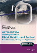
where is the spacecraft angular velocity with respect to an inertial frame I and expressed in body‐fixed frame B, and the unit quaternion describes the attitude orientation of the spacecraft in B with respect to I satisfying . Note that I₃ denotes the 3 × 3 identity matrix, and for , the notation denotes the following skew‐symmetric matrix:

(19.2)

Spacecraft dynamics:

When all the actuators run normally, the attitude control system is called a ‘normal’ system. Then, the dynamics of a rigid spacecraft can be described by:

(19.3)

where represents the positive‐definite moment inertia of the rigid spacecraft, is the control torque input generated by thrusters, and denotes the external disturbance torque.

In case of partial loss of actuator effectiveness, the system in Eq. (19.3) becomes a faulty one. In this chapter, the partial loss of actuator effectiveness is modelled by a multiplicative factor, and then the faulty spacecraft dynamic system can be rewritten as:

(19.4)

where denotes the effectiveness factor of spacecraft actuators, such that (). The case when means that the ith actuator works normally; for , it means that the ith actuator loses its effectiveness partially, but still works at all times.

For the development of control laws, the following assumptions are imposed:

The objective in this chapter is to design a fault‐tolerant control law for the system in Eqs. (19.1) and (19.4) such that the following targets are achieved in the presence of external disturbances and partial loss of actuator effectiveness:

• The closed‐loop system is globally stable, and in which all the signals are bounded and continuous.
• The attitude and angular velocity converge to an arbitrary small set containing the origin, that is, and .

In what follows, we shall develop such a control law for attitude stabilization of spacecraft.

19.3 Adaptive Backstepping Fault‐Tolerant Controller Design

In this section, for the normal system without an actuator fault, a baseline attitude controller based on the adaptive backstepping technique is developed. Then, using the baseline controller, the fault‐tolerant controller is derived. This guarantees that the actual outputs of the faulty actuators can still follow the normal command inputs, and the fault can be compensated online.

19.3.1 Baseline Attitude Controller Design

For the normal system in Eq. (19.3), let us introduce the following state variables transformation:

(19.6a)

(19.6b)

where α₁ is a virtual control law, which will be given latter. Then, the standard backstepping design procedure is elaborated as follows:

• Step1: Choose a Lyapunouv function candidate as
  (19.7)

  and select an appropriate virtual control α₁ as

  (19.8)

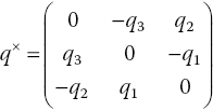
  where c₁ is a design parameter. Then, the derivative V₁ is

  (19.9)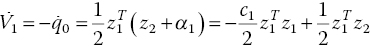

  Clearly if , then and z₁ is guaranteed to converge to zero asymptotically.

• Step 2. For the second error dynamic Eq. (19.6b) for z₂, one obtains
  (19.10)

  Now design the control input u as

  (19.11)

  By employing Eqs. (19.1) and (19.6), the derivative of α₁ can be calculated as

  (19.12)

  Choose a new Lyapunov function , and, in view of Eqs. (19.10)–(19.11), the time derivative of V₂ yields

  (19.13)

  where ε is a sufficiently small positive scalar control gain, β is an adequate positive constant, c₂ is a positive constant, and .

  Clearly, if   and , then , which implies that V(t) decreases monotonically. Therefore, the state signals are bounded ultimately as

  (19.14)

  which is a small set containing the origin ; moreover, the larger the values of c₀ and ε selected, the better control performance will be yielded. Using Eqs. (19.6) and (19.14), we have

  (19.15)

Thus, from Eqs. (19.13) and (19.15), it can be concluded that the closed‐loop system is globally stable. Then the following statements can be presented.

19.3.2 Adaptive Backstepping Fault‐Tolerant Attitude Controller Design

In Section 19.3.1, we used adaptive backstepping to designed a stable system for control of a spacecraft system with unknown disturbance torques. However, no actuator fault was considered. In this subsection, a partial loss of actuator effectiveness will be considered. To handle such a fault, for the ith actuator, the following auxiliary system is added:

(19.16a)

(19.16b)

(19.16c)

where and y_i are the input and output of the auxiliary system in Eqs. (19.16a)–(19.16c), respectively. Note that the output y_i is viewed as the actual output of the ith actuator, and the baseline controller in Eq. (19.11) is denoted u_nor. Then, the control objective in this sub‐part can be stated as: design control input for auxiliary system Eq. (19.16) satisfying Assumption 1 such that the output y_i can follow the specified desired signal , which represents the ith element of u_nor.

Before going into the details of the design of , the following definition and Lemma are presented:

Similar to the work of Zhang et al. [21], the following two filters are designed

(19.19a)

(19.19b)

where , , and matrix is strictly stable. Then, with the above filters, a state estimate for the system in Eq. (19.16) can be given by:

(19.20)

We define the estimation error as with . In view of Eqs. (19.16) and (19.20), one has:

(19.21)

From Eq. (19.21), the estimation error can be divided into two parts; that is, . Then:

(19.22a)

(19.22b)

From Eq. (19.22) and the definition of matrix A_i, one has

(19.23)

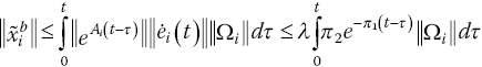
where π₁ and π₂ are chosen positive constants such that

(19.24)

Thus, we have

(19.25)

where the variable ζ(t) is the solution of the following equation

(19.26)

Due to the requirement of the strict stability of matrix A_i, there exists a positive definite matrix satisfying . Then, from Eqs. (19.16b) and (19.20), it follows that:

(19.27)

where x_i,2, are the second elements of the variables x_i, , respectively. Then, the auxiliary system in Eq. (19.16) can be rewritten in the following form based upon the designed filters in Eq. (19.19):

(19.28a)

(19.28b)

It can clearly be seen that Eq. (19.28) is written in a triangular nonlinear form. Hence, the standard backstepping controller design step can be implemented into it.

Take the state transformation as:

(19.29a)

(19.29b)

Where β_i is a virtual control law and will be designed later on. Now, the standard backstepping design procedures are adopted as:

• Step 1: From Eqs. (19.28a) and (19.19a), it follows that
  (19.30)

  Using the method of Zhou et al. [22], the virtual control law β_i is selected as

  (19.31)

  in which is a positive constant and χ satisfies the following equation:

  (19.32)

  and is selected as:

  (19.33)

  where m_i,1 and l_i,1 are two positive constants, and ê_i(t) and are the estimation of e_i(t) and λ, respectively. Then, with Eqs. (19.29), (19.30) and (19.33), one has

  (19.34)

  where .

  Then choose a new Lyapunov function as

  (19.35)

  where is a design parameter and .

  Using Eqs. (19.31), (19.32) and (19.34), the time derivative of V_i,1 can be calculated as

  (19.36)

  in which the Young’s inequality

  (19.37)

  is applied.

  From Eq. (19.25), it can be easily known that

  (19.38)

  Now design the update laws as

  (19.39a)
  (19.39b)

  where denotes the projection operator [25].

  Using Eqs. (19.37) and (19.38) and projection operator property [25] , , Eq. (19.36) can be rewritten as

  (19.40)

• Step 2. Now differentiating Eq. (19.29b) along with Eq. (19.28b), one has
  (19.41)

  where β_i is a function of , and can be calculated as

  (19.42a)

  Defining the Lyapunov function , the time derivative of V_i,2 yields

  (19.42b)

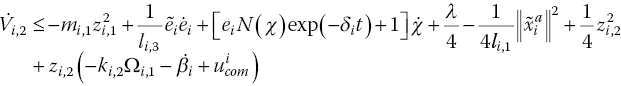
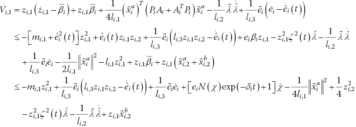
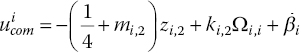
  Then the control input is designed as

  (19.43)

  Submitting the control in Eq.(19.43) into Eq. (19.42) yields

  (19.44)

  With the definition of V_i,2, it has

  (19.45)

  Integrating both side of Eq. (19.44) from zero to t yields

  (19.46)

  Then the following inequality can be achieved

  (19.47)

  where .

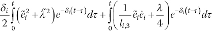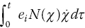  Note that because of the utilization of projection operator for ê_i(t) and , the boundness of and can be obtained. Then, incorporating with the boundness of and λ, it can be seen that is bounded. Thus, according to Lemma 1, V_i,2(t), and are bounded on [0, t_f). Therefore, z_i,1, z_i,2, e_i, λ and are bounded on [0, t_f) for all ; with Eqs. (19.16) and (19.29), it can be shown that all the signals in the closed‐loop system are bounded on [0, t_f) for all . Thus, according to Ryan [26], it can be shown that this conclusion is true for . Moreover, according to Eq. (19.47), one has

  (19.48)

  where

  (19.49)

  and the value of μ can be adjusted by appropriately choosing the design parameters. Based upon the above analysis, the following theorem can be concluded.

From Eqs. (19.48) and (19.49), it can be noted that the tracking error μ_i can be adjusted to a value as small as possible by appropriately choosing the parameters δ_i, m_i,1, m_i,2 and .

19.3.3 Fault Tolerance Analysis

From Eq. (19.16):

(19.50)

According to Theorem 2 and Eq. (19.48), it is reasonable to suppose that

(19.51)

where Δu_i satisfies the following inequality

(19.52)

Then under the effect of actual output of the ith actuator, the spacecraft dynamic can be rewritten as

(19.53)

where and satisfying .

From Eq. (19.50), Eq. (19.53) and the controller developed in Eq. (19.43), the whole attitude control system in the presence of a partial loss of actuator effectiveness can be depicted as in Figure 19.1.

In Eq. (19.53), the item can be viewed as the lumped disturbances. If the constant T_d is chosen as

(19.54)

then with the normal controller in Eqs. (19.11) and (19.53), the inequality in Eq. (19.13) can be guaranteed.

Therefore, based on Theorem 1, the following theorem can be obtained.

From the above analysis, because the matrix E is not used in the control scheme, there is no need to include a health monitoring unit to identify or estimate which actuator is unhealthy. The fault accommodation/compensation is done automatically and adaptively by the control algorithm. This feature is necessary to build affordable and effective fault‐tolerant spacecraft control schemes.

19.4 Numerical Simulations

In this section, the simulation results obtained using the control law in Eq. (19.43) are compared with conventional proportional‐derivative (PD) control, first for normal conditions and then then in the presence of the fault. The model parameters for the rigid spacecraft are chosen [15] as kgm² and the initial conditions Are set as and rad/s.

In the simulation, the external disturbance torque is assumed to be (Nm). In the actuator fault situation, the fault is assumed to be as in Eq. (19.55):

(19.55)

The time history of the fault is shown in Figure 19.2.

19.4.1 Simulations of PD Control under Normal and Fault Cases

In this simulation, a PD controller is implemented as the attitude stabilization control system, and it is of the form:

(19.56)

where design parameters and are selected in the simulation. The time histories of attitude quaternion, angular velocity and control input are shown in Figures 19.3a, 19.4a and 19.5a, respectively. We can clearly see that although the PD controller can stabilize the normal attitude within 8 s, it fails to stabilize the spacecraft when a fault leads to a partial loss of actuator effectiveness. Despite the fact that there is still some room for improvement with different design control parameter sets, there is not much improvement in the attitude and velocity responses.

19.4.2 Simulations of Proposed Control under Normal and Fault Cases

To show the effect of the proposed fault‐tolerant controller in Eq. (19.43), a simulation was performed under the same initial condition and fault scenario. In the simulation, the control parameters for the normal controller Eq. (19.11) were chosen as , , , and . For the fault‐tolerant controller, Eq. (19.43), the matrix P_i and the design parameters were set as:

The time responses of the closed‐loop system under the fault‐tolerant controller in Eq. (19.43) are shown in Figures 19.3b, 19.4b and 19.5b. Attitude stabilization can be achieved even with a fault leading to an unknown partial loss of actuator effectiveness. As expected, the attitude and the angular velocity will converge to an arbitrary small set containing the origin, as shown in Figures 19.3b and 19.4b. respectively.

The control input error Δu between the actual input u_act and the normal control signals u_nor is shown in Figure 19.6. The maximum value of Δu is smaller than 0.7. This together with selection of external disturbance d, leads to . Thus, is sufficiently large to deal with lumped disturbances, and so faults can be successfully managed with our proposed controller Eq. (19.43).

Summarizing both normal and fault cases, it should be noted that the proposed controllers have significantly better performance than the PD method in both theory and simulations. Also, in the presence of faults, the proposed methods are better than conventional controllers. In addition, extensive simulations were also done using different control parameters, disturbance inputs and even combinations of actuator faults. These results show that in the closed‐loop system attitude stabilization is accomplished in spite of these undesired effects. Moreover, the flexibility in the choice of control parameters can be utilized to obtain any desirable performance. These control approaches provide the theoretical basis for the practical application of advanced control theory to flexible spacecraft attitude control system.

19.5 Conclusion

A fault‐tolerant adaptive backstepping control scheme has been developed for spacecraft attitude stabilization in the presence of both an external disturbance and an unknown partial loss of actuator effectiveness. The proposed scheme does not require the system identification process to identify the faults. The control formulation is based upon Lyapunov’s direct stability theorem, incorporating the auxiliary system of the actual control output into the controller synthesis to compensate the actuator faults. The uniform ultimate bounded stability of the system is ensured and its robustness to both disturbance and actuator faults is also guaranteed.

The control designs are evaluated using numerical simulation and comparisons between the developed approach and other referred schemes, with the expected performance of the two being shown. In the simulation, different types of actuator failure scenarios were investigated. Based upon the results presented, it is concluded that the fault‐tolerant adaptive backstepping control scheme successfully handles failures if the efficiency of one or several actuators decreases. While the simulation results presented here merely illustrate formulations for attitude stabilization, further testing would be required to reach any conclusions about the efficacy of the control and adaptation laws for tracking arbitrary manoeuvres. In addition, this fault‐tolerant control scheme places no restrictions on the magnitude of the desired control, and designs where actuator limits are specifically considered are also being investigated.

References

1. 1 Bai X.L. and Junkins J.L., ‘New results for time‐optimal three‐axis reorientation of a rigid spacecraft,’ Journal of Guidance Control and Dynamics, 32 (4), 2009, pp. 1071–1076.
2. 2 Sharma R. and Tewari A., ‘Optimal nonlinear tracking of spacecraft attitude maneuvers,’ IEEE Transactions on Control Systems Technology, 12 (5), 2004, pp. 677–682.
3. 3 Hu Q.L., ‘Robust adaptive sliding mode attitude maneuvering and vibration damping of three‐axis‐stabilized flexible spacecraft with actuator saturation limits,’ Nonlinear Dynamics, 55 (3), 2009, pp. 301–321.
4. 4 Zheng Q. and Wu F., ‘Nonlinear H‐infinity control designs with asymmetric spacecraft control,’ Journal of Guidance Control and Dynamics, 32 (3), 2009, pp. 850–859.
5. 5 Li Z.X. and Wang B.L., ‘Robust attitude tracking control of spacecraft in the presence of disturbances,’ Journal of Guidance Control and Dynamics, 30 (4), 2007, pp. 1156–1159.
6. 6 Zhang Y.M. and Jiang J., ‘Bibliographical review on reconfigurable fault‐tolerant control systems,’ Annual Reviews in Control, 32 (2), 2008, pp. 229–252.
7. 7 Benosman M., ‘A survey of some recent results on nonlinear fault tolerant control,’ Mathematical Problems in Engineering, 2010, pp. 1–25.
8. 8 Zhang X.D., Parisini T., and Polycarpou M.M., ‘Adaptive fault‐tolerant control of nonlinear uncertain systems: an information‐based diagnostic approach,’ IEEE Transactions on Automatic Control, 49 (8), 2004, pp. 1259–1274.
9. 9 Zhang Y.W. and Qin S.J., ‘Adaptive actuator fault compensation for linear systems with matching and unmatching uncertainties,’ Journal of Process Control, 19 (6), 2009, pp. 985–990.
10. 10 Wang M. and Zhou D.H., ‘Fault tolerant control of feedback linearizable systems with stuck actuators,’ Asian Journal of Control, 10 (1), 2008, pp. 74–87.
11. 11 Boskovic J.D., Jackson J.A., Mehra R.K., and Nguyen N.T., ‘Multiple‐model adaptive fault‐tolerant control of a planetary lander,’ Journal of Guidance Control and Dynamics, 32 (6), 2009, pp. 1812–1826.
12. 12 Jung B., Kim Y. and Ha C., ‘Fault tolerant flight control system design using a multiple model adaptive controller,’ Proceedings of the Institution of Mechanical Engineers Part G – Journal of Aerospace Engineering, 223 (1), 2009, pp. 39–50.
13. 13 Lombaerts T.J.J., Smaili M.H., Stroosma O., et al., ‘Piloted simulator evaluation results of new fault‐tolerant flight control algorithm,’ Journal of Guidance Control and Dynamics, 32 (6), 2009, pp. 1747–1765.
14. 14 Ye S.J., Zhang Y.M., Wang X.M. and Rabbath C.A., ‘Robust fault‐tolerant control using on‐line control reallocation with application to aircraft,’ Proceedings of American Control Conference, New York, 2009, pp. 5534–5539.
15. 15 Cai W.C., Liao X.H., and Song Y.D., ‘Indirect robust adaptive fault‐tolerant control for attitude tracking of spacecraft,’ Journal of Guidance Control and Dynamics, 31 (5), 2008, pp. 1456–1463.
16. 16 Ji J., Ko S., and Ryoo C.K., ‘Fault tolerant control for satellites with four reaction wheels,’ Control Engineering Practice, 16 (10), 2008, pp. 1250–1258.
17. 17 Jiang Y., Hu Q.L. and Ma G.F., ‘Adaptive backstepping fault‐tolerant control for flexible spacecraft with unknown bounded disturbances and actuator failures,’ ISA Transactions, 49 (1), 2010, pp. 57–69.
18. 18 Godard, K.D. Kumar, and B. Tan, ‘Fault‐tolerant stabilization of a tethered satellite system using offset control,’ Journal of Spacecraft and Rockets, 45 (5), 2008, pp. 1070–1084.
19. 19 Zhang T.P. and Ge S.Z. S., ‘Adaptive neural control of MIMO Nonlinear state time‐varying delay systems with unknown dead‐zones and gain signs,’ Automatica, 43 (6), 2007, pp. 1021–1033.
20. 20 Marino R. and Tomei P., ‘Adaptive control of linear time‐varying systems,’ Automatica, 39 (4), 2003, pp. 651–659.
21. 21 Zhang Y.P., Fidan B., and Ioannou P.A., ‘Backstepping control of linear time‐varying systems with known and unknown parameters,’ IEEE Transactions on Automatic Control, 48 (6), 2003, pp. 1908–1925.
22. 22 Zhou J., Wen C., and Zhang Y., ‘Adaptive output control of a class of time‐varying uncertain nonlinear systems,’ Journal of Nonlinear Dynamic and System Theory, 5 (3), 2005, pp. 285–298.
23. 23 Sidi M.J., Spacecraft Dynamics and Control, Cambridge University Press, 1997, pp. 25–40.
24. 24 Ge S.Z. S., Hong F., and Lee T.H., ‘Adaptive neural control of nonlinear time‐delay systems with unknown virtual control coefficients,’ IEEE Transactions on Systems Man and Cybernetics Part B‐Cybernetics, 34 (1), 2004, pp. 499–516.
25. 25 M. Krstic, I. Kanellakopoulos, and P.V. Kokotovic, Nonlinear and Adaptive Control Design, Wiley, 1995, pp. 40–65.
26. 26 Ryan E.P., ‘A universal adaptive stabilizer for a class of nonlinear systems,’ Systems and Control Letters, 16 (3), 1991, pp. 209–218.