20
Novel Concepts in Multi‐rotor VTOL UAV Dynamics and Stability
Emaid A. Abdul Retha
Unmanned Vehicle University, Phoenix, AZ, USA
20.1 Introduction
The multi‐rotor is an unmanned aerial vehicle (UAV) lifted and propelled by two or more motors, usually electric, with propellers. The multi‐copter (as it is also called) is classified as a rotary UAV, which in contrast to fixed‐wing UAVs uses multiple rotating profiles or propellers for flight. This vehicle is characterized by a simple design with control of the craft delivered by varying the rotation of its rotors. In recent years, the perception of the uses of the multi‐rotor has increased due to its flexibility. It can to meet many of the requirements of vertical take‐off and landing (VTOL) UAVs for applications in reconnaissance and surveillance.
The different sites that need reconnaissance, surveillance and monitoring demand changes in the shape and configuration of VTOL UAVs, so as to guarantee operations in each set of special circumstances; for example, in narrow areas between buildings, in dense forests, in high winds and in areas of critical infrastructure with difficult and dangerous access. Effective multi‐rotor electromechanical design modifications can increase the under‐actuation of conventional multi‐rotors, leading to an increase in manoeuvrability and the ability to resist wind and fly in tight spaces.
The unmanned aerial system (UAS) industry is highly technological, and defines the development level of any state. The existence of a UAS industry requires development of the country’s infrastructure, including professional aviation educational institutions, high technology industries and highly skilled personnel in the industrial sphere. UASs are a promising and dynamic industry. UASs are in demand and are essential to cover a wide range of applications (military, security and civilian). UAS markets are very promising, and businesses involved can reach breakeven in reasonable periods.
UASs’ small size, remote or automatic control, low energy consumption, high safety in emergency situations, as well as the ability to use electric and alternative power sources, are characteristic.
The multi‐rotor VTOL UAV is a vehicle with many lifting rotors. Multi‐rotors are often equipped with fixed‐pitch propellers; control is achieved by varying the revolutions per minute (RPM) of each rotor. A quad‐rotor is a multi‐rotor with four rotors. A typical quad‐rotor is electronically controlled; there are also novel types that use additional means of control and these are referred to as electromechanically controlled quads. These will be the focus of this chapter, in which we will analyse novel concepts in multi‐rotor dynamics and stability, such as tilting rotors, variable pitch control and flap vector thrust, and consider how these concepts can be used to improve the quad‐rotor’s performance.
20.1.1 Motivation
Multi‐rotors in general, and the quad‐rotor in particular, have problems with their under‐actuation and autonomy. The problem of under‐actuation is related to the fact that the quad‐rotor has six degrees of freedom, but only four actuations (in other words, lift from the four variable rotors due to their variable RPM). This shortage is dealt with by increasing the actuations by adding electro‐mechanical controls. The energy required is stored in batteries, which are heavy and therefore limit the autonomy of the quad‐rotor. To solve this problem, a hybrid propulsion capability is required and the use of electro‐mechanical design allows this to happen, enhancing the vehicle’s autonomy.
Adding electro‐mechanical concepts to a multi‐rotor has many advantages:
- The quad‐rotor becomes a fully‐controlled system which can track any arbitrary trajectory; hovering with controlled pitch and roll angle, and motion with desired orientation.
- Navigation around obstacles in a cluttered environment is possible.
- Manoeuvring in only the horizontal plane is possible, useful for obstacle avoidance [1]; see Figure 20.1.
- Multi‐rotor input coupling can be achieved.
- The advantages of a 45° control method due to simultaneous cross‐coupling control of longitudinal, lateral in horizontal to all directions quad‐rotor’s movements can be demonstrated.

Figure 20.1 Quad‐rotor obstacle avoidance.
For a quad‐rotor to hover in the wind or move opposite to the wind’s direction, it is necessary to equal or overcome the drag forces: this happens by tilting the quad‐rotor’s body into the downwind direction. Logically, the higher the wind speed the higher the quad‐rotor tilting required; the tilting will keep increasing until the saturation of two motors opposite the wind direction is reached (they reach their maximum RPM). Therefore, in this chapter we will discuss this case and the use of electromechanical control: rotor tilting with either flap thrust‐vectoring control or with RPM control.
20.1.2 Review of Quad‐rotor Developments
In the last few decades, small‐scale UAVs have become common in many applications. Since the 1990s, with the development of microelectromechanical system (MEMS) technology, the multi‐rotor vehicle, especially the quad‐rotor vehicle, have been widely studied. The need for a UAV with greater manoeuvrability and hovering ability has led to the current rise in quad‐rotor research. The four‐rotor design allows quad‐rotors to be relatively simple in design, yet highly reliable and manoeuvrable. Cutting‐edge research is continuing to increase the viability of quad‐rotors by making advances in multi‐craft communication, environment exploration and manoeuvrability. If all of these developments can be combined, quad‐rotors will become capable of advanced autonomous missions that are currently not possible.
20.1.3 Contributions
The objective of this chapter is to highlight novel concepts in multi‐rotor dynamics and stability. It looks at a particular well‐developed quad‐rotor, which has been modified with specific electromechanical rotor controls to enhance its flying performance. The chapter will give:
- a full technical description of the modified quad‐rotor to overview the basic concepts
- a total mathematical model of the quad‐rotor, deriving kinetics and dynamics with regards to the addition of the electromechanical systems
- the basics of tilting quad‐rotor control, the control loops for each part of the control system and a state‐of‐the‐art mixing mechanism for tilting rotors (what is called a thrust‐vectoring quad‐rotor).
20.1.4 Chapter Overview
After this introduction, Section 20.2 is about general concepts of multi‐rotors, with a particular focus on the quad‐rotor, its mathematical modelling and its applications. Section 20.3 describes novel quad‐rotor concepts, types and designs, and the modelling and applications of electromechanical multi‐rotors. Section 20.4 provides some conclusions.
20.2 Multi‐rotors
The interest in UAVs for military and civil applications is growing fast; cheaper and more capable machines are in demand. Among the multi‐rotor layouts, the quad‐rotor has been widely chosen by many researchers as a promising vehicle for indoor and outdoor navigation. Multidisciplinary concepts are necessary because this type of rotorcraft attempts to achieve stable hovering and precise flight by balancing the forces produced by the four rotors. Nowadays, the design of multi‐copters with more than four rotors – the hexa‐copter and octo‐copter – is developing thanks to the possibility they bring of managing one or more engine failures and of increasing the total payload.
20.2.1 General Concept
The electronically controlled multi‐rotor, such as the quad‐rotor, has the components shown in Figure 20.2.

Figure 20.2 Multi‐rotor and its components: (a) propellers are usually fixed‐pitch; (b) airframe; (c) brushless motors are mounted rigidly to the airframe structure; (d) flight controller, stabilization board (containing an IMU, mainly mounted in a core hub section, communications, other assisting equipment, and parts for multi rotor control, stabilization and navigation); (e) landing gear; (f) payload; (g) radio control; (h) power (lithium polymer batteries); (i) ground station; (j) communications; (k) accessories.
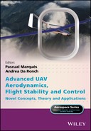
Electronically controlled multi‐rotors have several configurations (Figure 20.3 and Table 20.1).
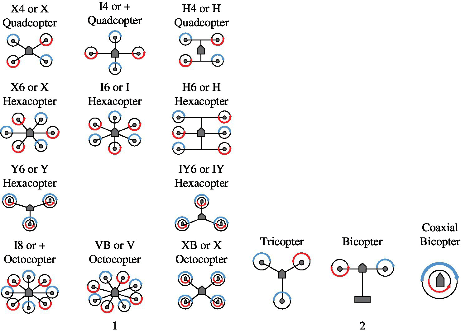
Figure 20.3 Multi rotor configurations: (1) conventional; (2) unconventional.
Table 20.1 Multi‐rotor configurations: advantages and disadvantages.
| Type | Motors | Coaxial | Advantages | Disadvantages |
| X4 or X | 4 | No | Simple and cheap | No redundancy |
| I4 or + | 4 | No | Simple and cheap | no redundancy |
| H4 or H | 4 | No | Simple and cheap | no redundancy |
| X6 or X | 6 | No | Limited redundancy and larger payload | Larger footprint and pricier |
| I6 or I | 6 | No | Limited redundancy and larger payload | Larger footprint and pricier |
| H6 or H | 6 | No | Limited redundancy and larger payload | Larger footprint and pricier |
| Y6 or Y | 6 | Yes | Small, high stability and wind resistance | Poor efficiency and complex |
| IY6 or IY | 6 | Yes | Small, high stability and wind resistance | Poor efficiency and complex |
| I8 or + | 8 | No | True redundancy and horsepower | large and expensive |
| V8 or V | 8 | No | True redundancy and horsepower | large and expensive |
| X8 or X | 8 | Yes | Very high lift capacity and wind resistance | Inefficient |
20.2.2 Quad‐rotor
Multi‐rotors, and in particular quad‐rotor configurations, have achieved their increasing popularity because of their mechanical simplicity, low cost and the availability of reliable components off the shelf. This makes them ideal for many mission scenarios. A quad‐rotor is regarded as a base design for multi‐rotor VTOL UAVs. Unlike most helicopters, quad‐rotors use two sets of identical fixed‐pitched propellers; two clockwise and two counter‐clockwise. Propellers use variation of RPM to control lift and torques, which are generated aerodynamically due to the propeller blades’ rotation. Control of vehicle motion is achieved by altering the rotation rate of two or more rotors, thereby changing the torque load and thrust/lift characteristics. More recently, quad‐rotors have become popular in UAV research. These vehicles use an electronic control system and electronic sensors to stabilize the UAV. With their small size and agile manoeuvrability, these quad‐rotors can fly indoors as well as outdoors. Flight control in electronically controlled quad‐rotors is achieved using a minimum of four control channels. One channel is usually the throttle, and increases or decreases power to all motors equally. This causes the aircraft to ascend or descend. The other three channels (as in radio control, called the aileron, elevator and rudder) control the roll, pitch, and yaw axes, respectively (Figure 20.4). These three control inputs work by causing a change in the quad‐rotor’s attitude (tilt or direction).
Figure 20.4 Quad‐rotor frames, forces, torques and control.
The main mechanical components needed for construction are the airframe, propellers (either fixed‐pitch or variable‐pitch) and the electric motors. For the best performance and simplest control algorithms, the motors and propellers should be placed equidistant. Recently, carbon fibre composites have become popular due to their light weight and structural stiffness. The electrical components needed to construct a working quad‐rotor are similar to those needed for a modern radio‐controlled (RC) electric helicopter. These are the electronic speed control module, on‐board computer or controller board and the batteries. Typically, an RC transmitter is also used to allow for human operator inputs.
Quad‐ and other multi‐rotors can often fly autonomously. Many modern flight controllers use software that allows the use of GPS to mark ‘way‐points’ on a map, to which the quad‐rotor will fly and perform tasks, such as landing or gaining altitude. The mathematical model of such an aerial vehicle represents a dynamical system with a 12‐dimensional state and 4‐dimensional inputs control.
20.2.3 Quad‐rotor Mathematical Modelling
For the mathematical modelling of novel concepts it is essential to start with a conventional quad‐rotor and then analyse electromechanical quad‐rotors as a development of them. By varying the motors’ speed and direction of rotation, the quad‐rotor can change its position and orientation. There are 12 (four groups × three parameters) states that describe the quad‐rotor’s dynamic behaviour:
- space position: P = [x y z]
- linear velocity: V = [ux vy wz]
- rotational angles: Ω = [φ θ ψ]
- angular velocities: ω = [pφ qθ rψ]
These values can be considered as the quad‐rotor’s outputs while the inputs are the applied forces and torques generated from the four motors’ rotation. The control model is shown in Figure 20.5. This shows the inputs and outputs for the quad‐rotor plant as a whole mechanical system. Generally, Newton’s second law of motion is working to represent the motion of the quad‐rotor [2].

Figure 20.5 Quad‐rotor control.
Therefore, the net force and the net moment acting on the quad‐rotor are written as:
where m is the quad‐rotor mass and I is the inertia matrix.
For a quad‐rotor, the lift force is distributed in four shares, one to each rotor and these forces are transmitted to the propellers (F1, F2, F3 and F4) according to the motor numbering (Figure 20.4). To find the values of these forces, the blade element momentum theory is used and they are a function of the rotation speeds of the propellers (denoted ω1, ω2, ω3 and ω4, to match the motors). The relationship used is Fi = k ωi2, i = 1, 2, 3, 4), where k is a proportionality coefficient). The thrust values depend on the propeller shape and air density, and so on. Other values affect the quad‐rotor, such as its mass (m) and weight (mg). It is natural that moments accompany propeller rotation (denoted M1, M2, M3 and M4), and their value is calculated as Mi = L × Fi, i = 1, 2, 3, 4, where L is the arm distance from the rotor axis to quad‐rotor centre of gravity (CG). It is very important to know the forces and moments to define the quad‐rotor modelling specifications, and to find the dynamic changes of these forces and moments is the foundation of quad‐rotor dynamic mathematical modelling, which in turn is the basis of quad‐rotor design and control [3].
The most important features of quad‐rotor design are:
- The reference systems (Figure 20.4), of which there are two:
- The Earth reference systems, or the Earth frame (xE, yE, zE).
- The quad‐rotor reference system, or the body frame (xB, yB, zB).
- The Euler angles(φ, θ, ψ), which define the transformation between the two systems:
- Roll φ: angle of rotation along axis xB to xE.
- Pitch θ: angle of rotation along axis yB to yE.
- Yaw ψ: angle of rotation along axis zB to zE.
- The angular speeds: the derivatives of (φ, θ, ψ) with respect to time are the angular rotation speeds of the system:
 Roll rate
 , Pitch rate
 , Yaw rate.
Analysis of quad‐rotor flight requires an elaborate mathematical model. The model needs to reflect the quad‐rotor’s behaviour in different flight phases (climb, descent, forward flight, manoeuvres, and so on). The mathematical model incorporates body motion dynamics and propulsion system aerodynamics. The propulsion system aerodynamics modelling tasks include: momentum theory, blade element theory, ground effect, vortex ring state and windmill break state. We need to know the quad‐rotor forces and torques, reference systems, Euler angles and angular speeds. We can then start assimilation of the process: the analysis, design and writing of the quad‐rotor mathematical model (the equations of motion). Analysis will be carried out on the various phases of the quad‐rotor’s flight.
- Hovering over a point Four conditions must be fulfilled:
- equilibrium of thrust: the sum of the rotor thrusts must equal the quad‐rotor’s weight
- no directional motion: the rotor thrusts are identical in each other’s direction as well as in the direction of gravity.
- balance of moments: the sum of moments equals zero.
- the sum of rotor rotation speeds equals zero:(20.3)Thus, the following conditions must be achieved:

 = 0,
= 0,  = 0,
= 0,  = 0; φ = 0, θ = 0, ψ = 0.
- Manoeuvres in the vertical direction There must be no equilibrium of thrust. The sum of the rotor thrusts does not equal the quad‐rotor weight. Euler angles and rates must also remain equal to zero.
Yaw rotation The sum of rotors rotation speeds is not equal to zero:
(20.4)
As a consequence: ψ =
 dt.
dt.Roll rotation To achieve quad‐rotor rolling we have to disturb the moment’s equilibrium, which is achieved by unbalancing propeller speeds:
(20.5)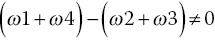
So φ =
 dt. This also means that the direction of all rotor lift forces does not act parallel to the direction of gravity g (no equilibrium of directions), so the quad‐rotor undergoes a roll through some angle. The roll rotation and translated flight means that the total thrust emanating from the quad‐rotor CG can be decomposed into a lift force = thrust × cos φ and drag force = thrust × sin φ. It is necessary to note here that in a roll manoeuver with further transition the quad‐rotor will slip down due to the lack of lifting thrust (the deficiency equal to F × sin φ). To avoid diving it is necessary that lift force = thrust × cos φ = −mg; so in translational flight we need more power to achieve hover or yawing (Figure 20.6). At this nominal hover state, the force produced from each propeller must satisfy:(20.6)
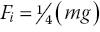
where Fi = k ωi2 ; motor speeds are given by:
(20.7)
Pitch rotation To make the quad‐rotor pitch, we have to disturb the moment equilibrium, which is achieved by unbalancing the propeller speeds:
(20.8)
So for pitching, (θ =
 dt). Also, by analogy to rolling, the total thrust is decomposed, so we need more power for quad‐rotor pitching.
Figure 20.6 Quad‐rotor roll rotation and translated flight.
Euler angle transformations are defined by ψ, θ and φ and a combined transformation matrix from body coordinates to the earth coordinates is obtained by three successive rotations (quad‐rotor kinetics).

where ‘c’ and ‘s’ denote ‘cos’ and ‘sin’ respectively. The Newtonian method is the most popular was of modelling rigid bodies with six degrees of freedom and has been used extensively for the modelling of many types of multi‐rotors. The derived model has six dynamic (three linear and three rotational) system equations (20.10) and (20.11):

where, CD1, CD2 and CD3 are drag coefficients, and (k (ω12 + ω22 + ω32 + ω42)) = u1 are the quad‐rotor control inputs. Euler equations are related to angular accelerations as follows:
where l is the distance of each rotor from the vehicle’s CG. Ix, Iy and Iz are moments of inertia along each of the axes and C1DR, C2DR and C3DR are rotational drag coefficients. Mi, (i = 1,2,3,4) are rotor moments produced by the angular velocity of the rotors and given by: Mi = Km ωi2; Km is a constant. u2 =k (ω42 − ω22), u3 = k (ω32 − ω12) and u4 = Km (ω12 − ω22 + ω32 – ω42), where u2, u3 and u4 are the angular quad‐rotor control inputs.
20.2.4 Quad‐rotor Applications
Despite their many uses, quad‐rotors can be categorized in a simple way as follows:
- Military and law enforcement Quad‐rotors are used for surveillance, reconnaissance, different intelligences, target acquisition, marches and demonstrations, and some sorties of dropping and delivery by military and law enforcement units, disaster and earthquake search and rescue missions in urban environments, geography and mapping.
- Civil The most notable of civilian applications are electric power line observation, geological or buildings survey, oil slick monitoring, communications, forest observation and meteorology services.
- Research and education The quad‐rotor is one of the most VTOL UAV requested and desirable at universities and research institutions involved in research related to control, stability, guidance and navigation. Modelling, simulations and new systems identification are also typical investigations.
- Commercial In the fields of sports, photography, cinema, hobbies and economically feasible projects such as quad‐rotor production for play and fun, which represents a wide public area.
20.3 Novel Quad‐rotor Concepts
Here we describe a patented quad‐rotor with tilting rotors, which built as a proof of concept of one type of electromechanically controlled quad‐rotor. This tilting quad‐rotor design is based on an electronically controlled conventional quad‐rotor. Therefore, we will first explain traditional quad‐rotors in a comprehensive manner, which will simplify the explanation of electromechanical control.
Electronical control of quad‐rotors entails the use of only the motors to control the attitude and transitions. This is the basic control for quad‐rotors but it is limited in performance because the vehicle is under‐actuated (there are four actuations to treat six degrees of freedom). To achieve innovative multi‐rotor VTOL UAV dynamics and stability, performance enhancements are required. This is achieved by increasing the actuations and adding electromechanical mechanisms to ensure improvements in multi‐rotor performance. The types, design, modelling and applications of different types of electromechanical multi‐rotors are discussed in the next subsections.
20.3.1 Electro‐mechanical Quad‐rotor
Multi‐rotor electromechanical designs have a variety of mechanisms of action. They are currently mostly trials or at the proof of concept stage: with the exception of the tri‐copter, they have not yet attained the popularity of pure electronic designs. The motivation for the use of electromechanical quad‐rotors is to address the shortcomings of conventional quad‐rotors for applications such as urban flights, obstacle avoidance, side slip imagery and windy‐flight capability.
20.3.1.1 Multi‐rotor with Variable‐pitch Propeller
These multi rotors utilize the same type of variable‐pitch rotor and swash plate as a conventional helicopter. This allows both very agile control and the potential to replace individual electric motors with belt‐driven rotors and propellers, which are hooked to a central electric motor or hollow‐shaft electric motor installed on each rotor arm’s end, with a control rod inside the hollow shaft to change the blade’s angle of attack. Internal combustion engines with belt drive can also be used; this is very important to enhance electric multi‐rotor performance parameters such as range and endurance. Variable pitch is not unusual, appearing in several multi‐rotor prototypes (Figure 20.7).

Figure 20.7 Different types of variable‐pitch propellers.
20.3.1.2 Multi rotor with Servo Thrust‐vectoring
The tilting of a rotor‐propeller vehicle, such as the bi‐copter, tri‐copter, and some multi rotor VTOL UAVs (Figure 20.8), utilizes both differential thrust and rotor tilting, with a servo mechanism to change its orientation. The bi‐copter and the tri‐copter are tilting‐rotor UAVs that are very popular alternative to electronically controlled multi‐rotors, which operate on pure lift by throttle control.
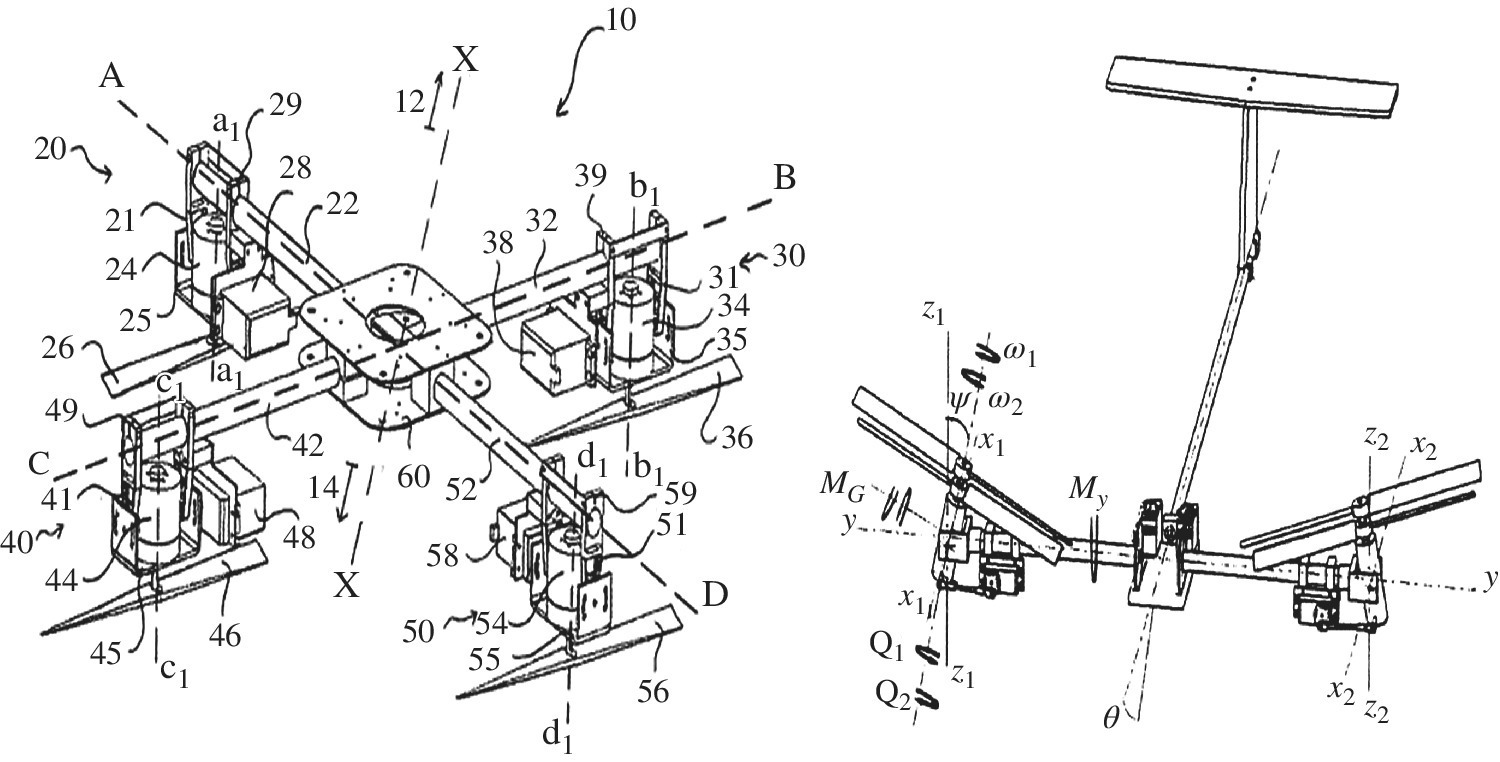
Figure 20.8 Different types of multi‐rotors with servo thrust‐vectoring.
Source: author’s patents (1) US 20130105635 A1; (2) US 20130105620 A1.
20.3.1.3 Flap Thrust‐vectoring
In fully actuated rotorcraft UAVs, whenever it is possible to rotate a motor‐prop combination or tilt rotors, it is also possible to redirect the flow using control vanes in the propeller downwash; in other words, using aerodynamically generated side force to drive the multi‐rotor to the desired direction. Flap thrust‐vectoring is not a common solution on commercial UAVs, but it is present in several custom‐built VTOL UAVs, and there are many promising research and production projects (Figure 20.9).
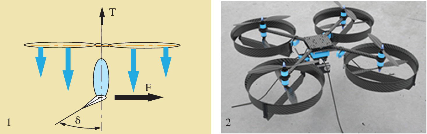
Figure 20.9 Flap thrust‐vectoring: left, principle; right, a design.
20.3.2 Variable‐pitch Quad‐rotor
In traditional fixed‐pitch quad‐rotors, stability and flight control are achieved by changing the speed of each of the four motors. While quad‐rotor differential RPM control is sufficient for most flight regimes and can result in agile and aggressive flight patterns, it places fundamental constraints on the vehicle as the flight envelope expands. In particular, control bandwidth is limited by the rotational inertia of the motors and fixed‐pitch quad‐rotors are unable to efficiently achieve reverse thrust. These constraints limit the aerobatic manoeuvers a quad‐rotor can perform, therefore limiting the future applicability of quad‐rotors in intensive agile missions. These limitations in fixed‐pitch quad‐rotors are overcome with the addition of variable‐pitch propellers. While variable‐pitch propellers add complexity to an otherwise simple and relatively robust quad‐rotor, the advantages of increased controller bandwidth and reverse‐thrust capabilities justify such a design when aggressive and agile flight is required (Figure 20.10).
Figure 20.10 Variable pitch quad‐rotor.
Controller bandwidth can be a significant problem for quad‐rotors, which is an issue for their stability as their size increases. Larger quad‐rotors require larger motors which, in turn, have larger inertias and cannot be controlled as quickly as smaller motors. Eventually, as the size increases sufficiently, the quad‐rotor can no longer be stabilized through RPM control alone because the torque required to change the rotational velocity of the motor quickly exceeds the capacity of the motor. Thus variable‐pitch blades may be necessary for larger quad‐rotors merely for stabilization purposes. The design of the variable‐pitch quad‐rotor in Figure 20.11 uses four digital high‐speed servos to control the pitch angle of the blade via a control rod that runs through a hollow motor shaft. Brushless motors are driven by electronic speed controllers. Inertial measurement, filtering, and high‐rate attitude stabilization is achieved using an autopilot, with combined optimum control achieved through simultaneous changes to propeller pitch angle and RPM of the motors.

Figure 20.11 Variable pitch rotors: top left, motor with hollow shaft; top right, motor with gear; bottom, variable‐pitch propeller design. Key: 1, servo‐machine; 2, ball bearing joint; 3, bearing; 4, hollow shaft; 5, brushless motor; 6, link bar.
Thrust actuation with fixed‐pitch propellers based on thrust produced by the propellers is almost constant with constant motor RPM (assuming the quad‐rotor is near hover). The way to change propeller’s thrust is by varying the voltage supplied to the motors, which varies propeller’s RPM. Adding variable‐pitch propellers to the quad‐rotor platform results in an additional degree of freedom in its actuation by changing the pitch angle of the propeller’s blade, thus varying the thrust produced by each motor‐propeller combination. With variable‐pitch propellers, thrust can be changed by either changing the blade pitch or by changing the rotational rate of the motors. These two actuations, to a large extent, can overlap. For instance, with variable‐pitch propellers the quad‐rotor can hover using high RPM and low blade pitch, or using low RPM and high blade pitch, or any combination in between. The output of the quad‐rotor attitude control loop is assumed to be a desired thrust. The lift force of each variable‐pitch rotor can be considered the rotor’s thrust and can be calculated using:
where, Ct is the thrust coefficient, ρ is the density of the air, n is the RPM of the motor, and D is the diameter of the propellers. The thrust coefficient is a function of the pitch angle of the propeller ϑ. The thrust coefficient in a linear (Ct = f (ϑ)) region can be calculated as:
where, is Ctϑ a derivative, which represents the thrust slope with respect to the variable pitch propeller (VPP) angle. This derivative is estimated using specialized software, which uses the number of blades, RPM, diameter of the propellers, and the velocity and the power of the motor. The value of Ct for an operational (VPP) angle range of 5° ≤ ϑ ≤ 15° is shown in Figure 20.12.

Figure 20.12 C t at different (VPP) angles.
Quad‐rotor VPP mathematical modelling uses the same proceedure as for conventional quad‐rotors except that the constant thrust of a fixed‐pitch propelleris replaced with the variable thrust as a function of the changing blade pitch and RPM, with the condition that VPPs have no tilt.
One recent attractive practical development of VPP quad‐rotors is the incorporation of internal combustion engines (ICEs) with hydrocarbon fuels. This will lead to marked increases in flight duartion (a weakness of electric quad‐rotors). With ICEs, different quad‐rotor or multi‐rotor configurations can be organised (Figure 20.13):
- single ICE (with generator), mechanical drive (belts or gears with shafts), multiple VPPs.
- multiple ICEs (with generators), direct drive, multiple or single VPP.
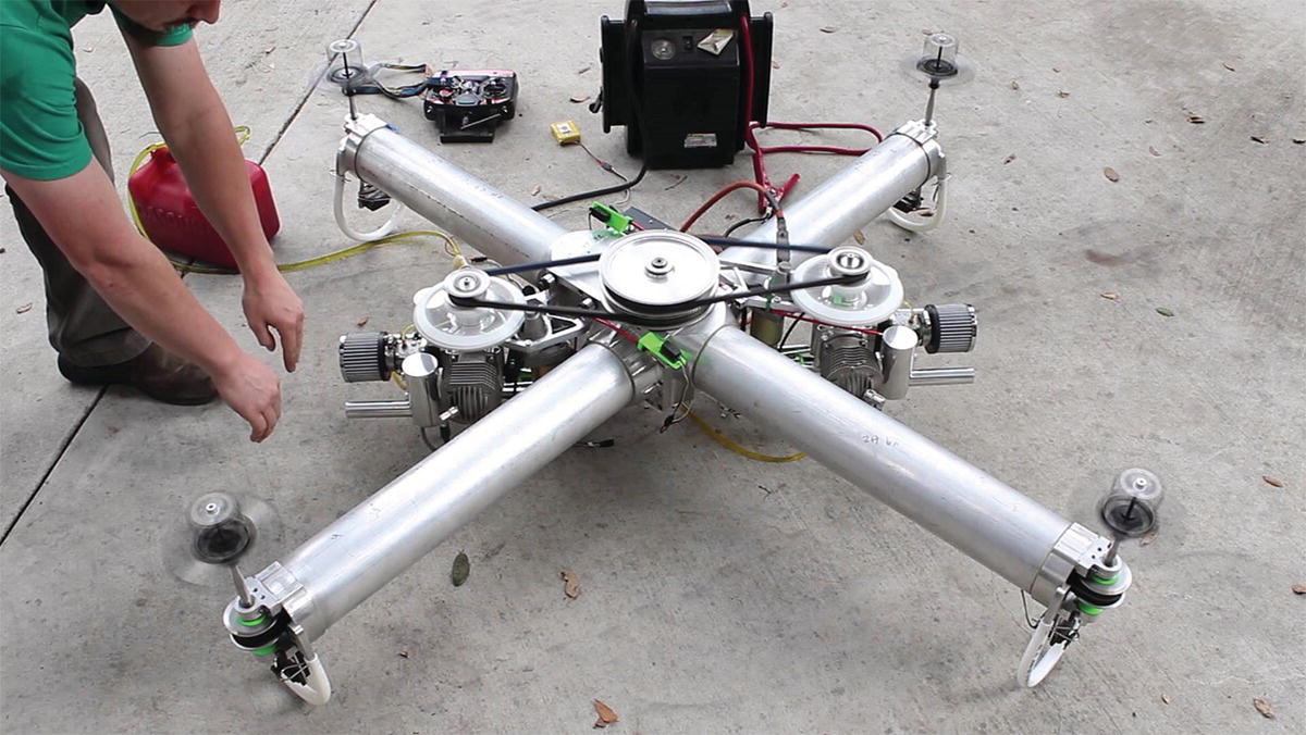
Figure 20.13 VPP quad‐rotor with ICEs.
20.3.3 Quad‐rotor Thrust‐vectoring
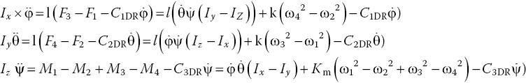
This section concerns a small tilt‐rotor VTOL UAV quad‐rotor; we will also use the term quad‐tilt‐rotor. The work is based on a patent by author ‘Quad tilt rotor vertical take‐off and landing (VTOL) unmanned aerial vehicle (UAV) with 45 degree rotors’. The patent is for a quad‐tilt‐rotor for research and proof of concept (Figures 20.8 and 20.14). Here we first discuss the quad‐tilt‐rotor design and its structure, and secondly we reflect on the quad‐tilt‐rotor’s modelling and control with regards to the specific impact of the tilting on the vehicle’s forces and moments as they directly affect the quad‐rotor dynamics and stability.

Figure 20.14 Quad‐tilt‐rotor component arrangement.
20.3.3.1 Quad‐tilt‐rotor Design
Quad‐rotor servo thrust‐vectoring or rotor‐tilting is a novel concept of multi‐rotor UAV control. Typical quad‐rotors are limited in their mobility and flight abilities because of their basic under‐actuation. The design motivation is to have a fully functional quad‐rotor without inclination of the body frame for those flight conditions that require a horizontal body frame and no stressed motor operation, such as when the quad‐rotor is confronting the wind horizontally; when minimum drag is the objective. The design should also ensure the correct position of the quad‐rotor’s CG, so that the trend line of the horizontal component passes through the CG; this avoids the generation of longitudinal and lateral moments because of the distance between the trend line and the CG is not equal to zero. Therefore, in some quad‐rotor designs motors with propellers are directed downwards; that is, the rotor is at a lower position. Also, the control algorithm is designed so that all the motors are able to tilt and/or rotate independently from each other.
The quad‐rotor prototype has the ability to control the alignment of its rotors, thus making it possible to overcome the under actuation and behave as a fully‐actuated flying vehicle. Driven by these limitations, a novel concept of a quad‐rotor UAV with tilting rotor‐propellers (propellers which can be actively rotated along the arm axes) is proposed. This will give full controllability of the quad‐rotor pose in 3D space. Developing this novel design, the goal is to transfer quad‐rotors from pure flying vehicles to fully flying robots with independent control over all six degrees of freedom of the main body and the ability to apply forces in arbitrary directions [4, 5].
The reason to choose a quad‐rotor with tilting rotors that is similar to a conventional quad‐rotor is that the equations of motion of the conventional quad‐rotor are simple and can help to reveal the differences needed to manage the required performance of the tilting quad‐rotor. Also, their mathematical model helps clarify the goals and benefits when rotor tilting is added to the design. In common with conventional quad‐rotors, the body frame consists of three main parts: central hub, carbon tubes (arms installation is at 45° relative to the x, y horizontal axes) and propulsion unit. In our case the fundamental difference is the propulsion unit. The electric motor is replaced with an electric‐motor tilting mechanism. The tilting mechanism contains the motor with the propeller, the clamp with swivelling device and the servo motor allowing the rotor to tilt in the plane perpendicular to the quad‐rotor arm at a certain angle (usually ±20°; Figure 20.14). This design gives convenient tuning, maintenance and replacement of parts.
The control of the quad‐rotor with such a tilting design is executed by two control loops: the first controls the rotation of the motors in a manner identical to conventional quad‐rotor; stability and motion are controlled by the quadrotor’s inclination as the motors are controlled by their RPM. The second control loop is to control the quad‐rotor transition in the horizontal plane (without inclination) in all directions. The transition is executed by tilting the rotors at different angles relative to the quad‐rotor arms (Figure 20.15); for example, to move the quad‐rotor accurately forward (along the x‐axis) we have to tilt the front rotors (rotors 1 and 2) inside towards the x‐axis and the backwards rotors (rotors 3 and 4) away from the x‐axis. If we need to move accurately right (along the y‐axis) we need to tilt the right rotors inside toward the y‐axis and the left motors away from the y‐axis. Logically if we need to move backwards or left the tilts are inversed. If we want to move to some in‐between direction, we must tilt the motors proportionally inside or outside; for example, if we need to move at 45° (forward and right) we tilt only rotors 1 and 3 inside the arm to the right; rotors 2 and 4 will be not tilted (in a flight test the quad‐tilt‐rotor combination showed very good matching). Note that quad‐rotor’s horizontal motion direction is the same as with tilted lift resultant inclination. To move quad‐rotor forward in the horizontal plane (XB–YB), the resultants with same (XB) direction will be added together for the four rotors and the resultants of each pair of motors in the YB direction will cancel (for four rotors their sum will be equal zero). This will result in the quad‐rotor moving forward.
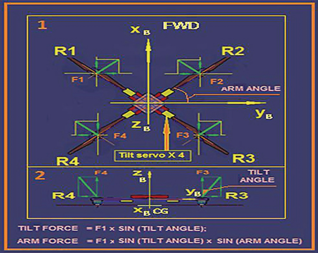
Figure 20.15 Quad‐tilt‐rotor principle with 45° tilting; (1) top view (2) side view.
When we needed to get full horizontal‐plane movement, the quad‐rotor’s CG vertical location must be at same level as the horizontal components of the lift force; otherwise, we will obtain inclined quad‐rotor motion (itself also a very interesting phenomenon for future analysis) due to an imbalance between the tilting force resultants’ moments (vertical and horizontal resultants). Mvert= Fvert × L, where L is the distance from the rotor to the CG, Mhor= Fhor × H, where H is the horizontal distance between the rotor and the CG. The first loop control will balance the propeller’s lift difference, which keeps the quad‐rotor in level flight. In other words, the distance is equal to zero, and there is no moment, so no disturbance for the first loop controller; meaning that the quad‐rotor moves level on the horizontal.
The basic concept of the novel quad‐rotor is to achieve over‐actuation (four spinning velocities plus four tilting velocities for a total of eight commands (shown in Figure 20.14 for one arm).
20.3.3.2 Quad‐tilt‐Rotor Modelling and Control
The first step in designing a control system for a given rotor vehicle is to derive a model that captures the key dynamics of this vehicle in the operational range of interest. Dynamic modelling is affected by the forces and torques that act on the flying vehicle. The conventional quad‐rotor, as an under‐actuated vehicle, has input from only the four lifting forces originating from the rotating propellers. Through adding tilting capability to all four rotors, the quad‐tilt‐rotor is over‐actuated, with eight actuators and six degrees of freedom.
From physics, we know that a tilting spinning body will generate different forces and torques. Therefore, it is necessary to present them:
- Force vector: The force generated by the quad‐rotor, which is the resultant force of the thrusts generated by the four propellers.
- Gyroscopic moments: Tilting of spinning propellers (rotation movements around two axes) creates gyroscopic moments that are perpendicular to these axes.
- Propeller torques: As the blades rotate, drag forces will be generated, which produce torques around the propeller’s aerodynamic centre. These torques act in the opposite direction to their direction of rotation.
- Thrust‐vectoring torques: These are the torques exerted by the force vector.
- Adverse reactionary torque: This torque acts when the rotor is suddenly tilted around certain axes. It depends especially on the propeller inertia and on tilting rate. The torque direction is opposite to the direction of tilting.
The dynamic model of the quad‐tilt‐rotor is derived by considering the vehicle as a rigid body that moves in a 3D space, through the main thrust and the pitch, roll and yaw torques. The quad‐rotor’s generalized coordinates are expressed as:
where the vector [x y z]T ∈ R3 (R: 3D space) corresponds to the position of the centre of mass of the quad‐rotor with respect to a fixed inertial frame. The [ψ θ φ]T ∈ R3 vector represents the Euler angles for the yaw, pitch and roll, around the x‐, y‐ and z‐axes respectively, which correspond to the quad‐rotor’s orientation in 3D space. The control of the quad‐tilt‐rotor is executed by two loops: first combine the quad‐rotor attitude control with motor RPM, quad‐rotor transition with quad‐rotor yaw control by differential motor RPM (that is, the first loop acts as a conventional quad‐rotor control). By the second loop, the quad‐rotor will transit strictly horizontally (x–y plane) without torques relative to the horizontal component of the lifting component direction. The arrangement of forces and torques is shown in Figure 20.16.
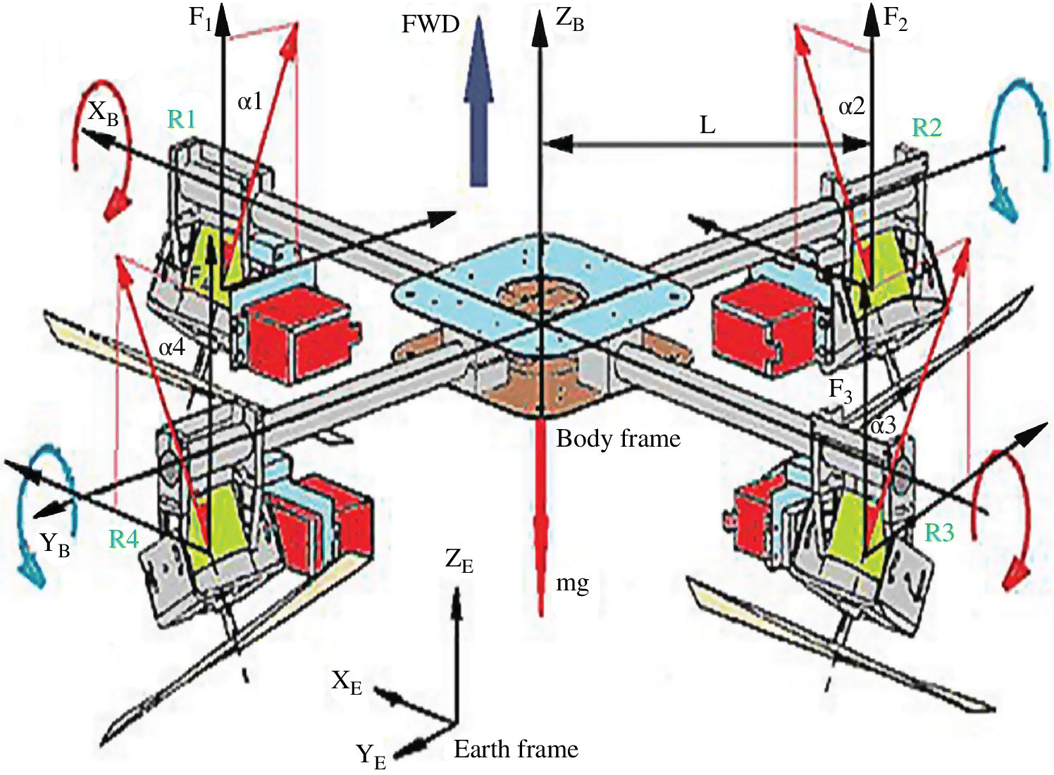
Figure 20.16 Quad‐tilt‐rotor: arrangement of forces and torques.
Under the assumption that the quad‐rotor is a rigid body, the CG is located in a plane of horizontal components (according to the requirements of translation in horizontal flight so that the CG location and quad‐rotor’s controller do not generate any torques). Gyroscopic moments are neglected to simplify the analysis of tilting effects. In Figure 20.15, we have two views of the quad‐rotor with the body and rotor systems of coordinates. Four rotors Ri (i = 1,2,3,4) tilt around the arms in the perpendicular plane at independent angles, with electric motors and propellers generating lift forces Fi (i = 1,2,3,4). Each rotor can tilt from vertical to an angle of 20° to either side. To explain how the tilting mechanism acts, we set the arm angle in this quad‐rotor design case to 45°; the tilt angle (α) and the motor have a lower position. In Figure 20.17, another of the author’s prototype designs shows the upper rotor arrangement.

Figure 20.17 Upper position of rotors.
Now we analyse whether forward transition is required (direction XB). First, assume a quad‐rotor in hover, so we have four equal lift forces Fi that in sum equal the quad‐rotor’s weight. Second, we tilt rotor 1 to the left and rotor 2 to the right; in other words, inside the forward arms at tilt angle = α = 0° ± 20°. Rotor 3 tilts to the right and rotor 4 to the left, outside the backward arms at tilt angle = α = 0° ± 20°). We have four tilted components; the vertical one equals Fi cos α, four horizontal components each equal Fi sin α, each of which is in turn divided into two components, the first parallel to axis XB (quad‐rotor’s arm force = Fi sin (±α)sin(±45°)), the second parallel to axis YB (quad‐rotor arm force = Fi sin(±α) sin(±45°). Components parallel to axis XB will be added and push the quad‐rotor horizontally forward; components parallel to axis YB will oppose each other and their sum will equal zero, which means that no side motion will take place (in the direction of YB). In the same manner, the quad‐rotor can transit to an arbitrary heading using different combinations of tilts (also, all moments for yaw are equal, so the quad‐tilt‐rotor experiences no yawing). Knowing the characteristics of the quad‐tilt‐rotor forces, we can now analyse the vehicle’s mathematical model.
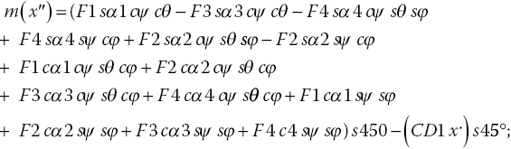
Generally Newton’s second law of motion (the Newton–Euler approach will be used) represents the motion of the quad‐rotor. Therefore, the net force and the net moment acting on the quad‐rotor are as in Eqs. (20.1) and (20.2). These dynamic equations could be obviously divided into translational and rotational equations of motion. For a quad‐tilt‐rotor, four more variables are included, which represent rotor combinations of tilting with angles αi. Regulation of these angles results in transition in all directions, which improves vehicle manoeuvrability, capability of hovering at a tilted angle and effectiveness in resisting the influence of the wind. It can be seen that rotor combinations are free to tilt around axes that are coincidental with the arm axes. The tilting rotors are slanted by angles αi relative to the vertical; αi (i = 1,2,3,4) is the tilt angle of the rotor. It is noted that the forces generated by the propellers are perpendicular to these particular planes of rotation, with regard to the previously mentioned rotational matrix and forces Fi (i = 1,2,3,4), and we can write translational equations of motion in the Earth frame as follows:

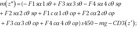
The rotational equations of motion are derived based on Euler equations:
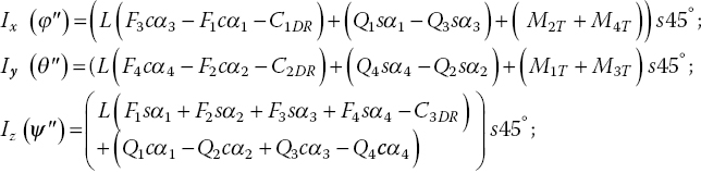
where m is the total mass of the quad‐rotor; g is the gravitational acceleration; x, y and z give the quad‐rotor’s position in Earth frame coordinates; CD1, CD2 and CD3 are drag coefficients; Fi (i = 1,2,3,4) is the rotor’s lift force; the 45° angle refers to the cross quad‐rotor design, with its arms at 45° relative to the body axes; L is distance of each rotor from the vehicle’s CG; IX, IY and IZ are moment of inertia around the x‐, y‐ and z‐axes, respectively; C1DR, C2DR, C3DR are rotational drag coefficients; Qi (i = 1,2,3,4) is the rotor moments due to their rotation; and MiT, (i = 1,2,3,4) is the tilt angle of reaction moments.
On the subject of quad‐tilt‐rotor control, it is necessary to address mathematical modelling and simulation, due to their importance in design, creation and development of any prototype. Modelling and simulation must be carried out in a certain sequence as this is important in the design process and the quality of the final product. Appropriate quad‐rotor mathematical modelling consists of two parts. First, we must design the quad‐rotor controller and, second, we must create a simulation model. Development of the controller is carried out by running the model through software such as MATLAB or SIMULINK with data from real flight tests on an actual flyable prototype (as in our case). The control performs a key role in the quad‐rotor’s stability, making it possible to control precisely the attitude and altitude states. Its main goal is to make the quad‐rotor move to a new desired position (called the ‘reference’) and also to react to external disturbances quickly and in a controlled way. Attitude control is the key element to maintain stability during flight. The quad‐rotor in space is represented through 12 state vectors, which are obtained by altering the mathematical model’s differential equations to the form:
where X = [![]() θ
θ ![]() ψ
ψ ![]() z
z ![]() x
x ![]() ]T; X is a state vector, U is the inputs vector; and T is the state space.
]T; X is a state vector, U is the inputs vector; and T is the state space.
Now if assume the main quad‐rotor dynamic system ![]() = f (X, U) is composed from two subsystems – the angular rotational and linear transitional Figure 20.18, top – we can see that three inputs (u2, u3, u4) affect six angular subsystems (six quad‐rotor attitude outputs: angles and angular rates). The other three inputs (u1, u5, u6) affect six linear transition subsystems (six quad‐rotor position outputs: coordinates and their rates or velocities). The u1 input acts on the electric motor’s thrust at vertical axes to change and maintain altitude. The u5, u6 inputs control the tilt of the rotor angles for steering and position changes in the horizontal plane. The transition subsystem also has attitude‐angle inputs to enhance dynamic response precisely; as the transition subsystem has output contain coordinates and their rates the quad‐rotor controller can operate dynamically. The lower part of Figure 20.18 shows the strategic control of the tilting quad‐rotor; it is the relationship between the input vectors (u2, u3, u4), input vector u1 and both linear transition vectors (u5, u6) with the quad‐rotor’s linear and rotational output parameters.
= f (X, U) is composed from two subsystems – the angular rotational and linear transitional Figure 20.18, top – we can see that three inputs (u2, u3, u4) affect six angular subsystems (six quad‐rotor attitude outputs: angles and angular rates). The other three inputs (u1, u5, u6) affect six linear transition subsystems (six quad‐rotor position outputs: coordinates and their rates or velocities). The u1 input acts on the electric motor’s thrust at vertical axes to change and maintain altitude. The u5, u6 inputs control the tilt of the rotor angles for steering and position changes in the horizontal plane. The transition subsystem also has attitude‐angle inputs to enhance dynamic response precisely; as the transition subsystem has output contain coordinates and their rates the quad‐rotor controller can operate dynamically. The lower part of Figure 20.18 shows the strategic control of the tilting quad‐rotor; it is the relationship between the input vectors (u2, u3, u4), input vector u1 and both linear transition vectors (u5, u6) with the quad‐rotor’s linear and rotational output parameters.
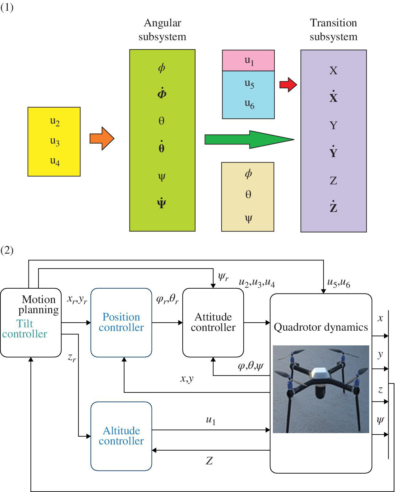
Figure 20.18 (1) Quad‐tilt‐rotor state vectors with input vector relationships (angular, transition subsystems); (2) Quad‐tilt‐ rotor control strategy.
The aim of this strategy is not only to control the position of the vehicle over a trajectory in three dimensions, as for a conventional quad‐rotor, but also to control its position in horizontal level hover and during path tracking. The controller inputs are the four independent speeds of the propellers and their tilt about the axes parallel to the quad‐rotor arms. Referring to Figure 20.19, we can see how four tilt servos mix for inclined control about the axes of tilting in the horizontal transition plane. In this case, we have three commands each one in two directions (normal and its opposite). The command could be received from a manual controller or from an autopilot; for conceptual understanding, suppose that commands can be given in pulse width modulation (PWM) format from minimum to maximum values or staying in the middle (neutral). The PWM commands, whatever their values, pass three mixers simultaneously (these mixers work using the same principle as the well‐known V‐tail RC mixer, namely two inputs and two outputs). The connections between commands, mixers and servos are organized in such way that the rotors will tilt in a direction that ensures the quad‐tilt‐rotor responds in such a way as to provide a horizontal plane level transition in any direction of motion or to face the wind in the horizontal plane by rotor tilting towards the wind.

Figure 20.19 Quad‐tilt‐rotor control with control mixing.
20.3.4 Flap Thrust‐vectoring
It is important for multi‐rotor VTOL UAVs to be able to change position without changing attitude and to maintain attitude without changing position, which is needed when flying in windy conditions. That cannot be achieved until the multi‐rotor has full actuation control. Above, we mentioned a configuration that allows an increase of actuation, namely rotor servo thrust‐vectoring or rotor‐tilting. However, there is another unique method for increasing multi‐rotor actuation: flap thrust‐vectoring. This method uses the flow stream from an upper positioned propeller to generate aerodynamic forces on the flap (or the vane) and to have a component directed horizontally, parallel to the propeller’s plane of rotation. These forces are used to control or steer the quad‐rotor in the same manner as the horizontal component of a tilt rotor [6].
From Figure 20.20, we note that the airfoil with a flap is blown by the propeller downwash to create aerodynamic force, while the flap is deflected (according to wing theory). These aerodynamic forces increase the actuation (more forces or servos make more degrees of freedoms). From wing theory, many factors affect the value of the aerodynamic force, such as airfoil shape, downwash velocity, flap deflection angle and flap surface area. As per the variable‐pitch propeller case, the aerodynamic forces can be calculated as follows:
where F is the generated aerodynamic force, ρ is the air density, V is the stream speed below the propeller; S is the airfoil total surface area; CL is air foil aerodynamic coefficient when the flap is deflected: CL = CLδ δ and CLδ is a derivative that represents the airfoil aerodynamic coefficient slope with respect to flap deflection angle δ.

Figure 20.20 Flap thrust‐vectoring principle and parameters.
The dynamical modelling is implemented as for servo thrust‐vectoring configurations, by reflecting in the mathematical model the relationship between flap deflection angles and the resulting forces and torques. Figure 20.21 shows flap thrust‐vectoring in a quad‐rotor.

Figure 20.21 Quad‐rotor with flap thrust‐vectoring: left, with props not shown; right, complete prototype.
20.4 Conclusions
UAVs of different shapes and sizes use electric propulsion systems to generate the required thrust. An efficient design of the propulsion system enhances performance, maximizes endurance, increases payload capabilities and prolongs the flight times of missions.
A conventional quad‐rotor mathematical model was presented as a basis for the model of a novel multi‐rotor (quad‐rotor) concept.
Different types of novel electromechanical quad‐rotors (variable‐pitch propellers, servo thrust‐vectoring; flap thrust‐vectoring) are described, focusing on servo thrust‐vectoring because of their common features.
State‐of‐the‐art electromechanical quad‐rotor mathematical modelling and their tilt‐mixing methodology was presented.
Based on our issued US patent [7] and research, and many successful flight tests of different quad‐tilt‐rotor prototypes, there is a good match of these quad‐tilt‐rotor concepts with the results of test flights, vehicle identification, and quad‐tilt‐rotor flight mixers for future autopilot developments.
We present the prospects for future research and developments projects, such as flap thrust‐vectoring.
References
- 1 R. Deits and R. Tedrake. Efficient mixed‐integer planning for UAVs in cluttered environments. IEEE International Conference on Robotics and Automation (ICRA), 2015.
- 2 P. Castillo Garcia, R. Lozano, and A. Dzul, Modelling and Control of Miniflying Machines, Springer, 2005.
- 3 S. Bouabdallah, Design and Control of Quad Rotors with Application to Autonomous Flying. PhD thesis, Ecole Polythechnique Federale De Lausanne, 2007.
- 4 M.‐D. Hua, T. Hamel, and C. Samson, ‘Control of VTOL vehicles with thrust‐direction tilting,’ in Proceedings of the 19th IFAC World Congress, 2014.
- 5 A. Gibiansky. Quadcopter dynamics and simulation. Blog post, Andrew.Gibiansky.com, 23 November 2012. URL: http://andrew.gibiansky.com/blog/physics/quadcopter‐dynamics/.
- 6 J. van den Berg, D. Wilkie, S.J. Guy, M. Niethammer, and D. Manocha LQG‐obstacles: Feedback control with collision avoidance for mobile robots under uncertainty. Web page 2011. URL: http://gamma.cs.unc.edu/CA/LQGObs/.
- 7 Quad tilt rotor vertical take‐off and landing (VTOL) unmanned aerial vehicle (UAV) with 45 degree rotors. US 2A1 (Patent).
Further reading
- 1 Sided performance coaxial vertical take‐off and landing (VTOL) UAV and pitch stability technique using oblique active tilting (OAT). US 2A1 (Patent).
- 2 E.A. Abdul‐Retha. UAV Propulsion Methods and Selection. Amazon, 2013.
- 3 E. Altug, J.P. Ostrowski and R. Mahony. ‘Control of a quadrotor helicopter using visual feedback,’ Proceedings of the 2002 IEEE International Conference on Robotics and Automation, pp. 72–77, 2002.
- 4 F. Archer, A. Shutko, T. Coleman, A. Haldin, E. Novichikhin, and I. Sidorov. ‘Introduction, overview, and status of the microwave autonomous copter system MACS,’ Proceedings of the 2004 IEEE International Geoscience and Remote Sensing Symposium, 2004.
- 5 R.W. Beard. ‘Quadrotor dynamics and control,’ Lecture notes, Brigham Young University, 19 February 2008. http://www.et.byu.edu/groups/ece490quad/control/quadrotor.pdf.
- 6 E.B. Nice. ‘Design of a Four Rotor Hovering Vehicle. MSc Thesis, Cornell University, 2004.
- 7 P. Harrop. Electric unmanned aerial vehicles (UAV) 2015–2025. Technical report, IdTechEx.