
15
Virtual Flight Simulation using Computational Fluid Dynamics
Ubaidullah Akram1, Marco Cristofaro2 and Andrea Da Ronch3
1 Lockheed Martin Commercial Flight Training, Sassenheim, the Netherlands
2 AVL List GmbH, Graz, Austria
3 University of Southampton, Southampton, UK
The aim of this chapter is to present recent advances in the development of high‐fidelity simulation software for virtual flight testing of unconventional and next‐generation aircraft. The accurate and efficient simulation of the full set of physics associated with aircraft flight operations, including flight control, aerodynamics and structural dynamics, is discussed. Pivotal to this framework is a novel adaptive design of experimental algorithms for the rapid generation of the aerodynamic database. This is developed and demonstrated on a complete aircraft with highly non‐linear aerodynamics. Throughout the chapter, several examples and problems are introduced to aid the reader to gain competence and proficiency in the methods and computer codes accompanying this chapter.
Section 15.1 overviews the state of the art of virtual flight simulation. Section 15.2 is a discussion of the aerodynamic model traditionally used for flight simulation. Then, surrogate modelling and adaptive design of experiment are developed in Section 15.3. Finally, advanced models used for virtual flight simulation are presented in Section 15.4.
15.1 Introduction
Many aspects of the detailed stages of aircraft design demand accurate understanding of the aircraft aerodynamics. Among other things, it is necessary to predict the static and dynamic characteristics of the aircraft, assessing performance and flight‐handling qualities, designing flight control laws and building aerodynamic models for flight simulation.
Obtaining reliable aerodynamic information throughout the flight envelope at the early stages of the aircraft design process is a difficult task. This is not always due to the limitation of the tools at the designer’s disposal but rather due to strict cost and time constraints, which encourage the use of the traditional design methods that are based on low‐fidelity, semi‐empirical and, mostly, linear formulations of aerodynamics originally developed for conventional aircraft configurations. Though computationally efficient and relatively accurate for flow regimes where the aerodynamics are predominantly linear, the traditional methods are unreliable for flight regimes involving complex non‐linear aerodynamic phenomena resulting from high angles of attack, increased rotational rates, flow separation, shock waves and their mutual interaction. For unconventional aircraft configurations, non‐linear flow fields can be encountered at low angles of attack in subsonic conditions and this raises questions over the applicability of the traditional methods, even for benign flight regimes. This often prohibits a detailed analysis of aircraft stability, performance and flight‐handling qualities, and camouflages possibly undesirable flight attributes during the initial stages of the aircraft design process. Discovering unwanted flight characteristics and control problems later in the design process can lead to programme delays, costly redesigns or retrofitting and ultimately degraded performance. There have been numerous examples of aircraft experiencing uncommanded activity, as reported, for example, in Chambers and Hall (2004).
High‐fidelity computational modelling and simulation can effectively provide virtual wind‐tunnel and flight testing. Flight simulation provides an alternative to traditional methods and can enable the modern aircraft designer to scan potentially unlimited design configurations. For this approach to be successful, a high‐fidelity aerodynamic model is imperative. However, building a high‐fidelity aerodynamic model requires high‐fidelity simulations, which are expensive in terms of computational cost and time. This chapter intends to introduce computational methods that can provide reliable aerodynamic information throughout the flight envelope and be cost and time efficient at the same time.
15.1.1 Flight Simulation
In the commercial aviation industry, flight simulation training devices are almost solely used for training pilots and maintenance personnel. In the academia, they find their major use as a research and teaching aid.
The scope of usage and performance of a flight simulation training device is determined by the level of its simulation fidelity. In the field of simulation, fidelity can be translated to realism: how close the simulation is to reality. A variety of flight simulation training devices exist, ranging from relatively low‐fidelity desktop trainers to full flight simulators that have the highest level of achievable fidelity; see Figure 15.1. A full flight simulator normally uses of actual aircraft hardware, from cockpit panels and flight controls to flight management computers, among others. Fidelity is further strengthened by a state‐of‐the‐art visual system linked to navigation databases, an extensive sound system and a motion system that can simulate complex atmospheric effects such as turbulence and buffet.


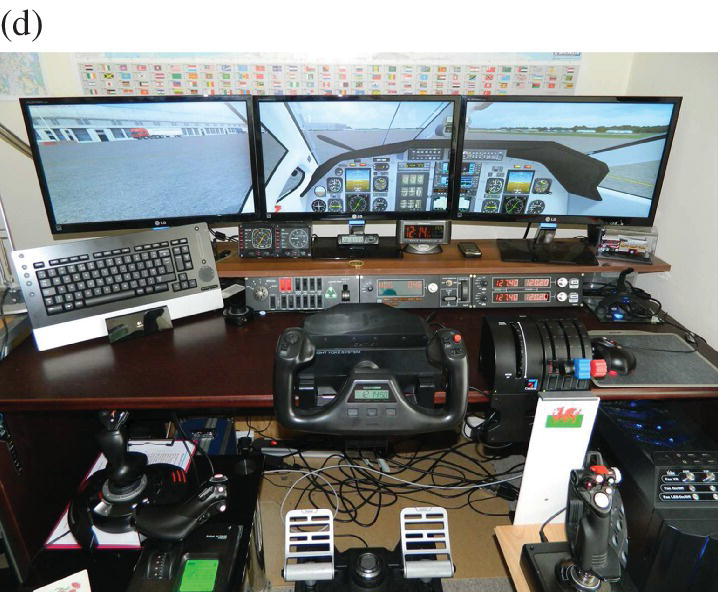
Figure 15.1 Examples of flight simulators: (a) B‐737 full flight simulator in a take‐off scene; (b) full flight simulator on motion; (c) FSC1000 desktop simulator; (d) hobby flight simulator.
(a),(b) courtesy Lockheed Martin Commercial Flight Training BV; (c) courtesy flightsimulatorcenter.com.
Not visible in Figure 15.1 is the software, which is a major component of any flight simulation training device. The software houses the system simulation, ground handling model and the flight dynamics calculations. The flight dynamics calculations are dependant on information about aerodynamic forces and moments, which are extracted from the aerodynamic model. When building a commercial flight simulation training device, the aerodynamic model is almost always supplied by the aircraft manufacturer. This aerodynamic model is first produced during the initial design stages and then improved as the design parameters are frozen and more information about the aircraft is made available. Finally, the aerodynamic model is further improved using data from wind‐tunnel and flight tests. This process is rather laborious and expensive.
For a flight simulation training device to be deemed fit for pilot training, it has to be certified by the governing aviation authorities, such as the Federal Aviation Administration or the European Aeronautical Safety Agency. The aviation authorities conduct a series of objective and subjective tests on the flight simulation training device before granting certification. Objective testing encompasses aircraft performance, stability and flight handling qualities. The aircraft manufacturer gathers and provides reference data to the flight simulation training device manufacturer for the objective tests in accordance with the guidelines defined by the aviation authorities. The reference data can either be from flight testing or from the aircraft manufacturer’s simulation. The flight simulation training device is then run using the same aircraft configuration and pilot inputs as the reference data. For each of the objective tests, the response of the flight simulation training device is required to lie within predefined tolerances of the reference data. If the response of the flight simulation training device does not fall within the tolerances, it will be deemed unfit for pilot training. The aerodynamic model, therefore, is critical to the fidelity of any flight simulation training device.
15.1.2 High‐fidelity Analysis for Conceptual Aircraft Design
Assessing performance, stability and flight‐handling qualities throughout the flight envelope during the conceptual design stages is not always possible. Often, this is a direct result of using traditional, low‐fidelity computational methods and standalone simulations, using, say, only two or three degrees of freedom (DoFs) or uncoupled calculations in order to minimise the cost and time. It is also important to mention that traditional design methods that rely on semi‐empirical formulations were developed for conventional aircraft configurations. As the industry pushes for unconventional designs, the applicability of these methods becomes questionable, even for benign flight conditions.
Flight simulation has the capability to facilitate a better conceptual design process. It can allow the designer to scan any aircraft configuration with a 6‐DoF model. This can improve the estimates obtained by semi‐empirical methods, allowing a better understanding of any coupled effects and enabling the designer to examine specific flight scenarios, such as those required for aircraft certification.
Further, if such a set‐up is to be better than the traditional approaches, it should be able to predict the performance, stability and flight‐handling qualities throughout the flight envelope. Fortunately, this can be achieved without the need for a high‐level flight simulation training device. An integrated desktop simulation and test environment is viable for the initial design stages. This has been successfully demonstrated by Scharl et al. (2000). However, this requires high‐fidelity mass properties information, an engine model, a ground handling model and an aerodynamic database. The intention of this chapter is to introduce a cost‐ and time‐efficient methodology to generate aerodynamic data for the complete flight envelope without compromising the accuracy of the predictions.
It is important to note that a comprehensive software tool (CEASIOM) has been developed to address these needs. The reader may find more information at http://www.ceasiom.com.
15.1.3 Aircraft Equations of Motion
The equations of motion of an aeroplane are the foundation on which the framework for flight dynamics studies is built. They provide the key to a proper understanding of flying and handling qualities. At their simplest, the equations of motion can describe small‐perturbation motion about trim only. At their most complex, they can be completely descriptive, simultaneously embodying static stability, dynamic stability, aeroelastic effects, atmospheric disturbances and control system dynamics for a given aeroplane configuration. The equations of motion enable the rather intangible description of flying and handling qualities to be related to quantifiable stability and control parameters, which in turn may be related to identifiable aerodynamic characteristics of the airframe. For initial studies, the theory of small perturbations is applied to the equations to facilitate their analytical solution and to enhance their functional visibility. However, for more advanced applications, which are beyond the scope of this chapter, the fully descriptive non‐linear form of the equations can be retained. In this case, the equations are difficult to solve analytically and computer simulation techniques become necessary to obtain a numerical solution.
Systems of Axes and Notations
The aircraft equations of motion are generally derived with respect to an inertial reference frame. In flight dynamics, the earth‐fixed reference frame is used, subject to a few assumptions, as the inertial reference frame. In the earth‐fixed reference frame, the XE ‐axis points towards north, the YE ‐axis towards east, and the ZE ‐axis is directed downwards (see Figure 15.2).

Figure 15.2 Systems of axes and notations.
The equations of motion may be referred to the aircraft‐fixed coordinate system. It is convenient to take the aircraft centre of mass as the origin of this coordinate system. Two sets of aircraft‐fixed coordinate systems are defined. The first is a pure translation of the earth‐fixed reference frame to the aircraft centre of mass, with axes denoted by XAE , YAE and ZAE (see Figure 15.2). This allows the position of the aircraft to be defined in terms of X, Y and Z coordinates. For the second coordinate system, the XAB ‐axis lies in the aircraft’s plane of symmetry and points forward, the YAB ‐axis is perpendicular to the aircraft’s plane of symmetry and is directed out towards the right wing, and the ZAB ‐axis lies in the aircraft’s plane of symmetry and points vertically downwards. This second coordinate system is commonly referred to as the ‘body‐fixed’ coordinate system and allows the orientation of the aircraft to be defined. Based on the chosen orientation of the X‐axis, different body‐fixed coordinate systems can be defined.
Governing Equations
The derivation of the aircraft equations of motion is detailed in any book on flight dynamics; see for example Napolitano (2011). The conservation law of linear momentum yields the three equations (15.1).

and the conservation law of angular momentum yields the three equations (15.2).

The left‐hand side of the above equations contains the external forces (FX , FY and FZ ) and moments (L, M and N) acting on the aircraft, and the right‐hand side describes the aircraft dynamics. It is of interest to observe that the external forces and moments may include contributions from the aerodynamics, thrust, ground operations and aircraft weight. This chapter, in particular, focuses on the computation of the aerodynamic loads using accurate yet rapid methods. However, before commencing the main task of this chapter, an overview of the underlying difficulties and research challenges is given.
15.1.4 Research Challenges
The impact of aviation on the environment is under scrutiny as never before, and both the EU and the USA have imposed strict targets on noise and emission pollution. These targets, however, are unlikely to be achieved by aircraft designed with current industrial design procedures, and considerable technological advances are desperately needed. To make progress in this direction, routine use of high‐fidelity coupled analysis will be required to improve realism of and confidence in the simulations. This will allow simulation of critical flight conditions, identifying undesired characteristics, and optimizing the overall performance well before the first prototype is built.
Based on the authors’ experience in the field of virtual flight simulation, three technical challenges should be addressed.
- efficient generation of the aerodynamic database for flight simulation
- integration of high‐fidelity computational models early in the aircraft design process
- data fusion of various aerodynamic sources to increase the realism and fidelity of the aerodynamic database.
Current state‐of‐the‐art methods and tools are discussed in light of the above three technical challenges. Advances beyond the state‐of‐the‐art form the core of this chapter, and will be thoroughly discussed in the remaining sections.
Efficient Generation of the Aerodynamic Database
To generate the aerodynamic database of forces and moments for the expected flight envelope, a large number of flow conditions must be calculated. Considering that the total number of flight conditions can easily be in excess of (106), the brute‐force approach of computing every entry becomes intractable using CFD as the source of the data. The issue of how to exploit the benefits of using CFD to improve aircraft design has been the topic of a large body of work (Da Ronch et al. 2011a; Mason et al. 1998; Snyder 1990). These papers exemplify the need for improvements in computational efficiency. Access to high‐performance computing (HPC) facilities is essential for numerous examples of intensive CFD simulations, but to make progress in routinely using CFD previous research has been concentrated on the development of computationally efficient predictive aerodynamic models combined with CFD simulations.
Despite the large body of work in this area, the formulation of an efficient, automated and robust method for the identification of aerodynamic non‐linearities has proven elusive. Most often, a large number of calculations is needed to ensure a good accuracy of the surrogate model. The slow convergence of the surrogate model may be attributed to the non‐optimal distribution of sample points over the flight envelope. As a result, CFD calculations are performed away from the areas where aerodynamic non‐linearities occur, missing critical features that may impact negatively on the design. The high non‐linearity of the aerodynamic force trends for a two dimensional case is presented in Figure 15.3. It illustrates the lift‐coefficient map for a domain based on the angle of attack and Mach number for a NACA 0012 aerofoil.

Figure 15.3 Lift‐coefficient dependency on angle of attack and Mach number for a NACA 0012 aerofoil.
This chapter discusses the formulation, development and implementation of a novel method to increase iteratively the accuracy of the surrogate model. The adaptive design of experimental algorithm has been found adequate to capture local maxima and minima, improving over state‐of‐the‐art methods, and satisfying the stringent constraint set on the maximum number of CFD calculations allowed within a given timeframe and without the use of exclusive HPC. This is presented in Section 15.2.1.
High‐fidelity Computational Models early in the Aircraft Design Process
Determining the stability and control characteristics of aircraft at the edge of the flight envelope is one of the most difficult and expensive aspects of the aircraft development process. Non‐linearities and unsteadiness in the flow are associated with shock waves, separation, vortices and their mutual interaction, which can lead to uncommanded motion and uncontrollable departures. If these issues are discovered at the flight test stage, the aircraft development can suffer significant delays, a rise in production costs and detrimental effects on performance. There have been numerous examples of aircraft experiencing uncommanded activity, as reported, for instance, in Chambers and Hall (2004). To provide a better fundamental understanding of the flow physics that might lead to degraded characteristics, computational approaches have been used (Woodson et al. 2005). The development of a reliable computational tool would allow the designer to screen different configurations prior to building the first prototype, reducing overall costs and limiting risks (Forsythe et al. 2006).
Probably, the most important drawback is that the aerodynamicist in conceptual design needs to project the potential performance of the design after a complete detailed aerodynamic design has been done. A CFD analysis of a shape that has not been designed is of no particular value. Indeed, a detailed wing design may take months to perform. The second drawback is the cycle time for CFD analysis. Despite the advent of more powerful HPC clusters, CFD analyses represent a bottleneck in the conceptual design process, which requires that several configurations be evaluated daily.
This chapter demonstrates that the routine use of CFD for conceptual design of complete aircraft is possible at a manageble cost. A key issue is a robust mesh generation tool; in this case it relies on the open software SUMO.1 SUMO is a graphical tool for rapid aircraft geometry creation, which is coupled to highly efficient unstructured surface and volume grid generators. It takes as input a very few basic geometry parameterization values and uses them to produce surface and volume grids for non‐viscous CFD simulations.
Data Fusion of Aerodynamic Sources
As the design process evolves from the preliminary to the conceptual phase, the aircraft geometry is tentatively frozen and experimental testing is started in order to corroborate and verify the aerodynamic predictions. With more detailed aerodynamic data being generated, it is necessary to incorporate the new information into the existing aerodynamic database, and so the fidelity of the database is iteratively enhanced during the aircraft design process. This approach, called data fusion, combines aerodynamic predictions from different sources to obtain one single database that is more accurate than each single database taken separately.
Two aerodynamic databases are incorporated or fused at a time. Generally, it is assumed that one database is of low‐fidelity/cost and the other one is of high‐fidelity/cost. The cheap evaluations of the low‐fidelity database provide information on the trend of the target function (qualitative behaviour), and expensive evaluations of the high‐fidelity database correct this trend with quantitative information. Because of the costs, the number of cheap evaluations is significantly larger than that of the expensive evaluations.
In practice, it may not be possible to set a clear separation between low‐ and high‐fidelity aerodynamic databases. For example, the data obtained from an expensive wind‐tunnel testing campaign might carry errors due to equipment limitations or external interference. Although the data may be generally not significantly affected, the flow field is much more sensitive close to the appearance of aerodynamic non‐linearities. In this case, an automated data fusion method seems not to exist to date, and engineering experience is still the most reliable guide.
15.1.5 Aircraft Test Cases
The methods described in this chapter were developed to address the need for a robust and systematic conceptual design tool for unconventional or next‐generation aircraft. Of special interest is the design of next‐generation aircraft that depart significantly from previous configurations. Existing conceptual design tools, which often rely heavily on correlations and fitted historical data, do not provide the flexibility or general performance prediction capabilities needed to address arbitrary new designs.
Two test cases of this chapter are for the Stability And Control Configuration (SACCON) and the Transonic Cruiser (TCR) wind‐tunnel models, shown in Figure 15.4.

Figure 15.4 The aircraft test cases of this chapter: (a)–(b) SACCON UCAV configuration (Vallespin et al. 2011); (c)–(d) TCR configuration. From Rizzi et al. 2011.
The SACCON model (Vallespin et al. 2011) is an unmanned combat air vehicle (UCAV) and consists of a lambda wing with a sweep angle of 53° and a wing washout of 5° (Figure 15.4a,b). The flow behaviour around this UCAV is characterised by vortical flows. A dual vortex structure is apparent up to about 17° angle of attack, when the dual vortices merge, causing strong non‐linear aerodynamic performance. The experimental data from the SACCON wind‐tunnel tests obtained in the 3.25 × 2.8‐m NWB wind tunnel for the rounded leading edge model (Loeser et al. 2010) are used in this chapter.
The design of the TCR model (Figure 15.4c,d), was made during the SimSAC project.2 The final configuration includes an all‐moving canard for longitudinal control. More details of the model design are given, for example, in Rizzi et al. (2011). The aircraft design is driven by the requirement for a design cruise speed in the sonic speed range. The specification for a cruise Mach number of 0.97 was set to stress the shortcomings of engineering methods traditionally used in the early design phase. A wind‐tunnel model was built and wind‐tunnel testing for static and dynamic conditions was performed in the facilities at the Central Aerohydrodynamic Institute (Mialon et al. 2010).
15.2 Aerodynamic Model for Flight Simulation
For flight simulation, a model of the aerodynamic forces and moments is required. The choice of an appropriate model is not unique, and may result from a compromise between the available information at the time and the turnaround time of simulations. In general, higher‐fidelity models of the aerodynamics are also more computationally expensive and require a complex geometry description. These competing aspects between accuracy, cost and time generally limit the complexity of models of the aerodynamics to simple relations, at least in the early phases of the aircraft development process and for multi‐disciplinary optimization analyses. Today, the most common model of the aerodynamics still relies on a model developed in the 1910s, albeit with minor modifications. Aircraft performance, however, has evolved considerably over the past 100 or so years, and the limitations of the traditional model are now becoming more and more apparent. The aerodynamic properties of an aircraft vary considerably over the flight envelope, and their mathematical descriptions are approximations at best. The limit of the approximations is determined either by the ability of mathematics to describe the physical phenomena involved or by the acceptability of the complexity of the description. The aim is to obtain the simplest approximation consistent with an adequate physical representation. In the first instance, this aim is best met when the motion of interest is constrained to small perturbations about a steady flight condition, which is usually, but not necessarily, trimmed equilibrium. This means that the aerodynamic characteristics can be approximated by linearizing about the chosen flight condition. Simple approximate mathematical descriptions of aerodynamic stability and control derivatives then follow relatively easily. This is the approach pioneered by Bryan (1911), and it usually works extremely well provided the limitations of the model are recognised from the outset. But real flight does not obey mathematical limitations.
15.2.1 Tabular Aerodynamic Database
Modeling the aircraft aerodynamics raises the fundamental question of what the mathematical structure of the model should be. The functional dependencies of the force and moment coefficients are in general complex, as they depend non‐linearly on present and past values of several quantities, such as airspeed and angles of incidence. The flow is often considered quasi‐steady, which presumes that the flow reaches a steady state instantaneously and that the dependence on the history of the motion variables can be neglected. One exception to this assumption is the retention of reduced‐frequency effects. With these underlying hypotheses, the characterization of the functional dependencies is broken down as:

The first term on the right‐hand side can be obtained in steady‐state analyses and static wind‐tunnel tests; the second term represents Reynolds number corrections and the last two terms are measured from rotary balance and forced oscillation tests, respectively. The decomposition is valid when the effects are separable and the superposition principle is valid. The effects of rotary and forced oscillations are typically modeled as a function of the body axis angular rates, angles of incidence and their first time derivatives. These derivatives were introduced to obtain a closer correlation between predicted and observed aircraft longitudinal motion, and for a conventional aircraft they represent the finite time that aerodynamic loads at the tail lag the changes in downwash convected downstream from the wing.
Traditionally, data obtained from extensive wind‐tunnel and flight‐test campaigns are tabular in form, expressing the dependencies of the aerodynamic loads on the flight and control settings. This form also represents the standard format used in flight simulators, for stability and control assessment, and for flight control system design and synthesis. As illustrated in Table 15.1, forces and moments are tabulated as functions of the aircraft states and control settings. Aerodynamic coefficients are in wind axes, and the aircraft states feature the angles of incidence and sideslip, α and β, the Mach number, M, and the body‐axis angular rates, p, q and r. All required control deflections are also included. Several assumptions have led to the formulation used, limiting its validity when confronted with uncommanded departures involving aerodynamic and aircraft motion cross‐coupling.
Table 15.1 Aerodynamic database format.
| α | M | β | δ ele | δ rud | δ ail | … | p | q | r | CL | CD | Cm | CY | Cl | Cn |
| × | × | × | — | — | — | — | — | — | — | × | × | × | × | × | × |
| × | × | — | × | — | — | — | — | — | — | × | × | × | × | × | × |
| × | × | — | — | × | — | — | — | — | — | × | × | × | × | × | × |
| × | × | — | — | — | × | — | — | — | — | × | × | × | × | × | × |
| × | × | — | — | — | — | × | — | — | — | × | × | × | × | × | × |
| × | × | — | — | — | — | — | × | — | — | × | × | × | × | × | × |
| × | × | — | — | — | — | — | — | × | — | × | × | × | × | × | × |
| × | × | — | — | — | — | — | — | — | × | × | × | × | × | × | × |
× indicates a column vector of non‐zero elements.
Typical Size of the Tabular Model
In the general case, the six aerodynamic coefficients would be functions of all input variables, resulting in a very large table (see Section 15.3). This is not normally necessary, and a less coupled formulation of the aerodynamic coefficients is used instead. Each aerodynamic term is formulated as dependent on three input variables. The main aerodynamic variables are taken to be the angle of attack α, and Mach number M. Forces and moments are assumed to depend on these variables in combination with each of the remaining variables separately. The complete aerodynamic database is then divided into three‐parameter sub‐tables. Let nx denote the number of values for the parameter x in the table, and let Nc denote the number of aircraft control effectors. The dimension of the complete database, ndb , is as follows
where ωi indicates the body axis angular rates.
For the same example illustrated above, the total number of table entries would be less than 200. However, a reasonable aerodynamic database to cover the expected flight envelope can easily require 100,000 entries.
15.2.2 Stability‐derivatives Approach
The functions f 1, f 2, f 3 and f 4 shown in Eq. (15.3), represent the dependency between aerodynamic forces and moments coefficients, and states and command variables. These are the integral result of the pressure distribution over the aircraft surface for every state condition. The stability‐derivatives approach linearizes these functions, so that the motion of the aircraft can be more readily analyzed. These derivatives are measures of how forces and moments change as states and command variables change.
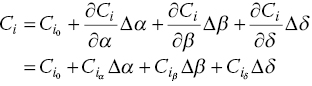
Start by considering only the steady part of Eq. (15.3), f 1. Variations in forces and moments with reference to an initial condition of equilibrium, for a certain Mach number, can be expanded using a Taylor series and expressed as in Eq. (15.5).
Neglecting higher order terms, the equation is linearized as follows:
![]() is the f
1 gradient term in the α direction and is one of the so called ‘aerodynamic derivatives’. Based on whether a derivative reflects a change in force or moment based on an aircraft state or a control surface deflection, they are referred to as stability and control derivatives, respectively.
is the f
1 gradient term in the α direction and is one of the so called ‘aerodynamic derivatives’. Based on whether a derivative reflects a change in force or moment based on an aircraft state or a control surface deflection, they are referred to as stability and control derivatives, respectively.
Static Aerodynamic Derivatives
Whereas the linear superposition of the effects above is considered adequate for most conventional aircraft configurations, unconventional geometries exhibit highly non‐linear dependences on control deflections, even at benign flow conditions for their particular configuration layout. As an example, consider the SACCON test case (Figure 15.4), which has been the subject of extensive numerical investigations and wind‐tunnel testing. Both the numerical predictions and wind‐tunnel measurements indicate the development of a complex flow field, which results in the principle of superposition being invalid. More accurate and non‐linear models of the aerodynamics are therefore sought, in order to improve the simulation of the next generation of aircraft.
Equation (15.5) also assumes that the aerodynamic forces and moments are an instantaneous function of the aircraft states and control variables. For flight manoeuvres involving slow angular rates and linear angle‐of‐attack regimes, the flow adapts relatively quickly and can be reasonably assumed to be independent of time (Vallespin et al. 2010). However, the time‐invariance assumption is not true for manoeuvres involving high‐angular rates and angles of attack where non‐linear and unsteady aerodynamic effects are dominant.
Consider Figure 15.5, representing the flow field around SACCON during a pull‐up manoeuvre designed to take the aircraft through the non‐linear angle‐of‐attack regime in a short period of time: the angle of attack changes from −5 to 30° in about 1 s. The two different flow fields are steady (Figure 15.5a) and unsteady time‐accurate (Figure 15.5b) CFD calculations, respectively. The surface topology of SACCON results in vortex formation at the leading edges, indicated by the darker regions. For the steady case, the vortices are stronger and break down further downstream relative to the unsteady time‐accurate case. During such manoeuvres, the flow characteristics are actually a function of the previous motion history of the aircraft. This is known as aerodynamic hysteresis, in which the aerodynamics become time dependent. This time‐variant phenomenon has been extensively investigated for aerofoils, wings and for full aircraft configurations (Mueller 1985; Venkatakrishnan et al. 2006). In this non‐linear flight regime, the model predictions have been shown to degrade (McCracken et al. 2012; Vallespin 2012) and provide erroneous indications of the aircraft behaviour.

Figure 15.5 SACCON surface pressure distribution during a pull up manoeuvre, at M = 0.1026 and α = 26.3° (Vallespin et al. 2010).
Dynamic Aerodynamic Derivatives
The aerodynamic predictions obtained via the stability‐derivatives approach for non‐linear and unsteady flight regimes can be improved by adding motion rates terms f 3 and f 4 from Eq. (15.3). These additions, referred to as dynamic derivatives, were introduced to obtain a close correlation between predicted and observed aircraft longitudinal motion (Greenberg 1951).
For each aerodynamic force and moment, as we did for the steady flight condition, we can retain the linear terms that are most relevant and de‐couple their combined influence into individual contributions. Most aircraft are symmetric and this property can be used to our advantage to neglect the dependence of longitudinal forces and moments on lateral‐directional variables and vice versa. While the dependence on β is typically neglected for a quasi‐steady flow, the inclusion of the ![]() term leads to an identifiability problem when estimating the
term leads to an identifiability problem when estimating the ![]() and q derivatives (Da Ronch 2012). To avoid this problem, the two terms are lumped together and an equivalent derivative is defined as
and q derivatives (Da Ronch 2012). To avoid this problem, the two terms are lumped together and an equivalent derivative is defined as ![]() for i = L, D and m.
for i = L, D and m.
Following from the discussion above, we present a non‐linear mathematical formulation for the longitudinal and lateral aerodynamic forces and moments in quasi‐steady flow, as presented in Eq. (15.7).

where i = L, D and m and j = Y, l and n.
The static aerodynamic contributions and the dynamic derivatives can either be determined through measured or computed aerodynamic data. A discussion of the available methods is presented in Section 15.2.3, while the dynamic derivatives are discussed in Section 15.3.6.
15.2.3 Sources of Aerodynamic Predictions
A prerequisite for realistic predictions of the stability and control characteristics of an aircraft is the availability of a complete and accurate aerodynamic database. The choice of which aerodynamic model to use balances cost and fidelity. The higher the fidelity of the aerodynamic model to be used, the higher the execution time normally is. In the early phases of aircraft development, the geometry is defined with limited fidelity, which might render expensive methods of limited use. A number of models are used and these are now summarized.
Figure 15.6 shows knowledge available and resources committed at various stages of the aircraft design process. The methods developed in this chapter aim at bringing higher‐fidelity tools, that are generally used only in the later stages of the development process, into use early in the design cycle. The benefits of doing so are to bring significant insights from increased realism of the complex non‐linear interactions that may jeopardise the aircraft performance, and to improve the aircraft design well before it changes become economically unfeasible.

Figure 15.6 Increasing fidelity and cost of the aerodynamic model during the aircraft design process.
Semi‐empirical Methods
Semi‐empirical methods, which are the traditional engineering tool for conceptual design, often rely heavily on correlations and fitted historical data, and do not provide the flexibility or sufficiently general performance prediction capability to address arbitrary new designs. The data compendium (DATCOM), for example, is a document of more than 1500 pages, covering detailed methodologies for determining stability and control characteristics of conventional ‘wing–fuselage’ aircraft configurations. In 1979, it was programmed in Fortran and renamed the ‘USAF stability and control digital DATCOM’ (Williams and Vukelich 1979). Digital DATCOM is a semi‐empirical method that can rapidly produce the aerodynamic derivatives based on geometry details and flight conditions. This code was primarily developed to estimate aerodynamic derivatives of conventional configurations, and to provide all the individual component contributions and the aircraft forces and moments. A design uncertainty factor is often needed to account for validity of aerodynamic characteristics estimated using this method. Figure 15.7 shows the level of simplification of the geometry used by DATCOM.
Figure 15.7 Geometrical representation of a traditional aircraft in DATCOM.
Numerical Methods
CFD provides a range of methods, with varying fidelity, that can be employed for aerodynamic analyses of aircraft. The Navier–Stokes (NS) equations that describe the motion of a viscous and compressible flow form the basis of any CFD analysis. The underlying non‐linear partial differential equations have to be solved numerically with appropriate algorithms, and provide the highest level of fidelity. NS computations are also the most computationally expensive. Reduced‐fidelity equations can be achieved through simplification of the NS equations. On the other end of the fidelity spectrum, the linear potential flow theory is the most computationally efficient but its generality is strongly limited to linear cases.
Full aircraft configurations can be analysed using high‐fidelity CFD (McDaniel et al. 2010). This can provide a better understanding of flow physics throughout the flight envelope and this has been successfully demonstrated in the literature (Woodson et al. 2005; Ghoreyshi et al. 2010). However, the computing cost and time required for high‐fidelity CFD analysis of full aircraft configurations across their flight envelope limits its use in the initial design process.
The error between low‐ and high‐fidelity CFD computations for benign flight conditions is usually negligible. However, for flight conditions where non‐linear flow characteristics are dominant, this error increases considerably. Therefore, a combination of low‐ and high‐fidelity CFD analyses enables the cost‐ and time‐efficient generation of aerodynamic databases for aircraft. The low‐fidelity analyses are used for benign regions of the flight envelope, while high‐fidelity analyses are used for extreme flight conditions. Figure 15.4b shows the surface pressure coefficient around the SACCON configuration at two angles of attack. The resulting aerodynamic forces and moments are integrated from the surface pressure distribution.
Wind‐tunnel Testing
Before the Wright brothers managed to take their Flyer I off the ground more than 100 years ago, they had performed a series of careful experiments with different wing models in a small wind tunnel installed in their bicycle shop. Since then, many successful aircraft have been designed in an increasingly more complex process, involving both experimental and analytical or computational models. Testing a new design, or a component of it, in wind tunnels or by using mathematical models is necessary because of the high risk and considerable costs involved in producing and flight testing a prototype. With more and more complex aircraft, longer development cycles and immense development costs, the need for reliable, accurate, and practical modelling increases.
Wind‐tunnel testing provides realistic measurements to validate and verify the accuracy of simulations and to investigate critical effects that are not capture in simulations. However, wind‐tunnel tests suffer from issues such as blockage, scaling, mount interferences and Mach/Reynolds number effects (Beyers 1995). The disadvantages of wind‐tunnel testing are as follows:
- Designing and manufacturing a fully equipped wind‐tunnel model and running the experimental campaign is very expensive and time consuming. The costs and time scales involved in testing do not meet the requirements of conceptual and preliminary aircraft design, where the speed of the investigations and flexibility in new aircraft designs are needed.
- For wind‐tunnel testing, an aircraft configuration is required. If the geometry is not finalised, testing is of little value. Wind‐tunnel testing remains too expensive and time‐consuming to provide useful indications to the aircraft designer, and it is usually performed in the later stages of the aircraft development process when the flexibility in the design changes is limited.
- Wind‐tunnel testing is limited by physical constraints, affecting the range of flight conditions to be tested. Dynamic tests, in particular, are limited by the weight and size of the wind‐tunnel model.
Figure 15.8 shows the wind‐tunnel models of the SACCON and TCR models mounted in the test facilities. The scaled models were tested at low and high speeds for both static and dynamic cases.

Figure 15.8 Wind‐tunnel testing.
Flight Testing
Flight testing is the process of developing and gathering data during operation and flight of an aircraft and then analysing that data to evaluate the flight characteristics of the aircraft. Flight‐test assessments take place in areas which include, but may not be limited to, the following:
- Aircraft performance: Aircraft performance comprises stall‐speed measurement, climb rates and gradients, cruise range and endurance, descent or glide rates and gradients, and take‐off and landing distances.
- Flight handling: Aircraft flight‐handling qualities include stability, controllability and manoeuvrability, trim, and stalling and spinning characteristics.
- Aircraft systems: Piloting and operational features of aircraft controls, systems and avionics, such as the human–machine interface. Assessment of aircraft instrumentation and independent test instrumentation used during flight testing is also included.
- Human factors: Ergonomic, workload and operational environment aspects.
Flight testing is certainly the most accurate and expensive method to obtain information about a test aircraft. Not only is an aircraft prototype needed, but also high risk is involved with testing; see Figure 15.9. Flight testing has been traditionally used to improve the aerodynamic predictions obtained through other methods. Parameter identification techniques have been used extensively to obtain aerodynamic coefficients for aircraft. The general idea behind parameter identification is to minimize a pre‐defined error between the measured and modelled aerodynamics. Corrections obtained through this error minimization process are then applied to the modelled aerodynamics to improve the match with the flight‐test‐measured parameters.
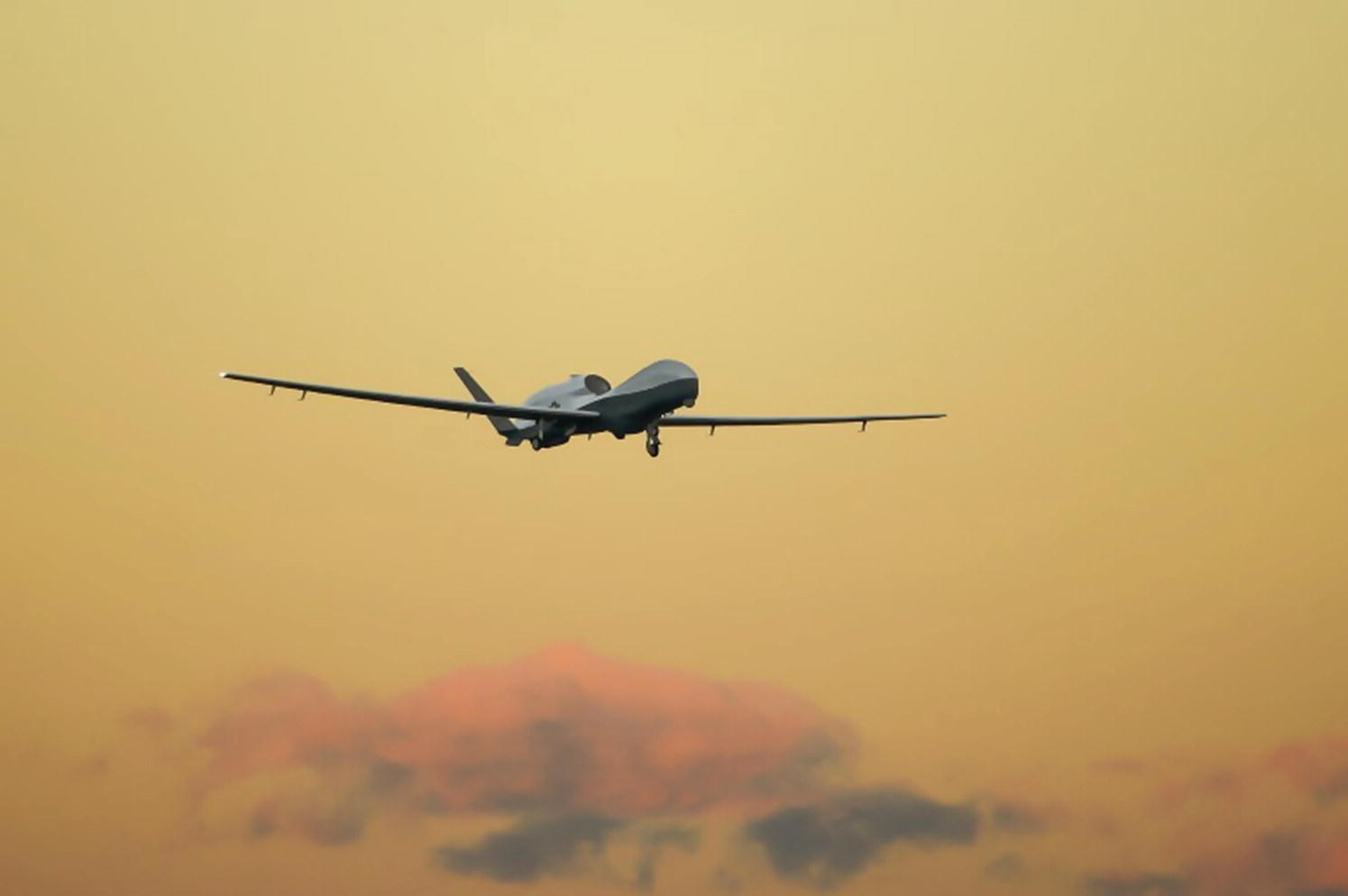
Figure 15.9 The MQ‐4C Triton test aircraft makes its approach for landing at Palmdale, California, marking the conclusion of initial flight testing.
Image: Alan Radecki.
15.3 Generation of Tabular Aerodynamic Model
Refer to Table 15.1 and consider an aircraft with three traditional control surfaces (elevator, aileron and rudder). Then, assume a coarse approximation of the flight envelope that consists of ten samples uniformly distributed for each parameter range. The parameter space in this case spans nine dimensions: three flight conditions, three control settings and three angular rates.
Two situations may arise. The first situation is when there is a requirement to deliver a table detailing the complete dependence of the aerodynamic coefficients on the nine parameters. In this case, the tabular aerodynamic model consists of 109 entries, which corresponds to a matrix of 10 billion rows and 15 columns (nine parameters and six aerodynamic coefficients). The second situation is for a requirement of a less coupled representation of the aerodynamic coefficients, as discussed in Section 15.2.1. In this case, using Eq. (15.4), the size of the tabular aerodynamic model is 7000 entries (reduced from 10 billion in the first situation).
This section discusses efficient methods to generate high‐dimensional large tabular models, as exemplified by the problem above.
15.3.1 Brute‐force Approach
The costs of computing every single entry of the tabular model are prohibitively expensive. For the problem above, assume that a single prediction of a rapid numerical model takes about 10 s, inclusive of pre‐ and post‐processing times. When used for to the smaller case of 7000 entries, the generation of the full tabular model would require nearly 20 hours of computing time: an unreasonable time.
When using the brute‐force approach in combination to high‐fidelity aerodynamic models to fill the tables, an unrealistic time of 158 years has been suggested (Rogers et al. 2003). An alternative to the brute force approach is based on sampling, reconstruction and data fusion of aerodynamic data, as fully discussed in the following section.
15.3.2 Surrogate Model
Kriging Model
Kriging generates an interpolation model for non‐linear and multi‐dimensional deterministic functions. In Cristofaro et al. (2014), Mackman et al. (2013) and Zhang et al. (2013) the Kriging interpolation is used to reduce the computational cost of generating a full aerodynamic model. Once the Kriging model is created, it becomes a computationally cheap model for prediction of the function at untried locations.
Consider the three‐dimensional table for an aerodynamic force/moment coefficient with the independent variables being α, M and β. To begin, the range of the independent variables for use in the aerodynamic data table is defined and initial data sample locations are selected to lie along the boundaries of the three‐dimensional parameter space. Latin Hypercube Sampling (Giunta et al. 2003), a modification of the well‐known Monte Carlo method (Hastings 1970), is then used to obtain a few additional data sample locations within the parameter space. The aerodynamic force/moment coefficient is then computed for these data locations. The idea is that this initial sampling will provide a quick overview of the variation of the aerodynamic force/moment coefficient throughout the parameter space and help, as described next, to identify additional data sample locations.
Kriging is then used to interpolate data at untried locations – that is, where data is not available – throughout the parameter space. Based on predefined criteria, a new data sample location is selected in one of the untried points and the process then repeats until a predefined tolerance on the criteria is met. Selection of the initial data sample locations at the boundaries removes the risks of extrapolation.
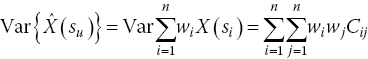
Kriging predicts the values at untried locations using a weighted average of the values at the available data sample locations. It is different from the other weighted‐average interpolation methods in that it assumes that the parameter being interpolated for is a random variable; this ensures that the expected value of the prediction error is 0 and it minimizes the variance of the prediction error. Let X = [X 1, X 2, …, Xn ] be a vector representing data at known data sample locations s = [s 1, s 2, …, sn ]. Kriging assumes that the random variable can be written as:
where f(si ) is usually called the mean and represents a trend (constant, linear or quadratic) and Z(si ) represents a stochastic process with variance σ 2.
Various modifications of Kriging interpolation method are available in the literature (Cressie 1991). Cristofaro (2014) and Ghoreyshi et al. (2009) employed universal Kriging, which assumes f(si ) is non‐constant and a function of the data sample locations. For universal Kriging, where each data sample location can be characterized by p parameters:
f (si ) has to be defined to solve the universal Kriging equations. Ideally, this would be dictated by the physics of the problem. Often, the trend is unknown and is usually modelled as a lower‐order polynomial of the coordinates of the design sites. The Kriging prediction, at an unknown location su , can be written as:

where ![]() is the predicted value and wi
are the weights to be computed. Note that wi
are allowed to vary for different predictions.
is the predicted value and wi
are the weights to be computed. Note that wi
are allowed to vary for different predictions.
The prediction error at the unknown location, su , can be written as:
where ![]() is the prediction and X(su
) is the random variable modelling the true value. Note that the prediction error is also a random variable since it is a linear combination of random variables.
is the prediction and X(su
) is the random variable modelling the true value. Note that the prediction error is also a random variable since it is a linear combination of random variables.
For the expected value of R(su ), E{R(su )}, to be 0:

Substituting for E{X(si )} and E{X(su )}, we can re‐write Eq. (15.12) as:

Let us assume that the mean, f (si ), is a linear function of α, M and β. This allows us to write:

Substituting Eq. (15.14) into Eq. (15.13) we find that, for E{R(su )} to be 0, we require:

which basically requires  .
.
As mentioned earlier, Kriging also attempts to minimize the variance of the prediction error. The variance of a weighted linear combination of random variables can be written as (Isaaks and Srivastava 1989):

Applying Eq. (15.16) to Eq. (15.11), we can write:
The first term in Eq. (15.17) describes the covariance of ![]() with itself and is equal to the variance of
with itself and is equal to the variance of ![]() . Since
. Since ![]() is a linear combination of random variables, applying Eq. (15.16) to
is a linear combination of random variables, applying Eq. (15.16) to  yields:
Similarly, the last term in Eq. (15.17) describes the covariance of X(su ) with itself and is equal to the variance of X(su ). As mentioned earlier, the random variables modelled by Kriging are assumed to have variance σ 2. Hence:
The remaining two terms in Eq. (15.17) can be lumped together as ![]() and simplified as follows:
and simplified as follows:
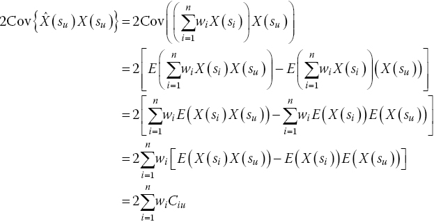
Note that the derivation of this equation makes use of the theorem (Isaaks and Srivastava 1989) that ![]() .
.
Combining the expressions from Eqs. (15.18)–(15.20), we can write the expression for the variance of the prediction error as:

The minimization of Eq. (15.21) is a constrained problem, with constraints given in Eq. (15.15). To find a solution, the method of Lagrange multipliers is used to transform this constrained problem into a unconstrained one (Isaaks and Srivastava 1989):
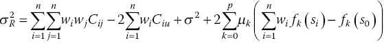
The error variance presented by Eq. (15.22) can be minimized by setting the first partial derivatives of n + p + 1 equations with respect to wi and μk to 0. This results in the n + p + 1 equations which can be written in the form Ax = B as follows:

where:
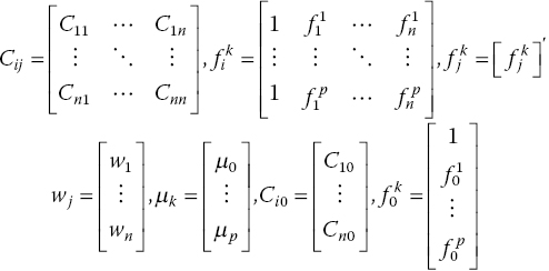
To solve the universal Kriging equations, a covariance model for the data is required. Several covariance models are available in the literature, see for example Isaaks and Srivastava (1989).
Example 1
This example demonstrates a simple use of the Kriging model. It shows how an interpolation model can be obtained and how it can be used to compute the approximate value of the function at a chosen point. Let us start by considering a one‐dimensional function X = f (s), the value of which is known only at n specific points. The target of the Kriging model is the evaluation of the function in unsampled locations.
Given a set of n = 3 design sites, s = [s
1, …, sm
] = [−2, −1, 3], and responses X = [X
1, X
2, X
3], we aim to compute the value ![]() in su
= 0. A schematic representation of the problem is given in Figure 15.10.
in su
= 0. A schematic representation of the problem is given in Figure 15.10.

Figure 15.10
Problem domain; the known data are X
1, X
2 and X
3 and the unknown is  .
.
A covariance, or correlation, model is needed to describe the relationships among variables. So consider a linear model defined as R(d) = max{0, 1 − θ · d} with d the relative distance. We take the parameter θ = 1/6 = 0.167, so that all the considered points influence each other. Since the smaller the value of θ, the wider is the influence of the known data over the domain, this value needs to be chosen after considering the nature of the problem. The resulting values of the covariance model are then presented in Table 15.2.
Table 15.2 Values of a linear covariance model with θ = 1/6.
| d | 0 | 1 | 2 | 3 | 4 | 5 | 6 | … |
| R(d) | 1 | 0.833 | 0.667 | 0.5 | 0.333 | 0.167 | 0 | 0 |
The matrix with the covariance model values between the sampled locations, C, is then needed. The elements indicate the respective correlation between different sampled points Cij = R(|xi − xj |). Equation (15.24) shows how the correlation matrix is created within this example. The C matrix is square, with dimension n × n and it is dependent on the norm of the distance between sample points, explaining its symmetrical nature.

As done with C, a covariance vector D(su ) between sampled points and a generic unknown point su , must be generated, as showed in Eq. (15.25). The elements indicate the influence of known data on the unknown point Di = R(|si − su |). Considering su = 0, the first element is D 1 = R(|s 1 − su |) = R(2) = 0.667.
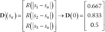
It is now possible to find the weights of the available samples on the unknown points, w. The theory gives the resulting formula, as presented in Eq. (15.26), where 1 is a column vector of ones of size n.
It is important to notice that since C is not a function of su , the inversion of the matrix is necessary only once, even when many estimations are required.
The resulting weights are then presented in Figure 15.11. The resulting values in su
are then easily computed as ![]() .
.

Figure 15.11 Resulting Kriging model weights in s 1, s 2 and s 3 associated with su = 0.
Now consider two other data cases: one linear with X = [0, 1, 5] and one parabolic with X = [0, 1, 25]. The resulting values ![]() in su
= 0 are respectively 2 for linear and 7 for parabolic, as shown in Figure 15.12.
in su
= 0 are respectively 2 for linear and 7 for parabolic, as shown in Figure 15.12.

Figure 15.12 Example of the Kriging interpolation for a parabolic and a linear function with a linear covariance model.
The reader is finally invited to reflect on the following points:
- Since we used a linear correlation model, for the linear case the predicted value is actually coincident with the real value.
- In the parabolic case, the predicted value is a linear interpolation between the values at 0 and 3. In this case the Kriging method neglects the point at −2, giving a weight there of 0 for su = 0.
Example 2
In this example, we illustrate the use of Kriging to iteratively refine the sample space for the lift coefficient of the NACA 0012 airfoil in the α − M domain. Let us consider angles of attack ranging between 0° and 14° and Mach numbers between 0.3 and 0.7.
Figure 15.13 presents a schematic of the UniversalKriging code, which can be found in the ancillary material to this chapter. To begin with, a total of six sample points are selected, four of which lie at the boundaries and two of which are selected to lie in the regions where we expect non‐linearities. The points at the domain boundaries allow extrapolation to be avoided. The two other points can be selected via a Monte Carlo simulation. However, if a priori knowledge of the physical phenomenon governing the sample space is available, these points can also be selected through engineering judgement, as in this case. Table 15.3 presents the details for the initial samples.
Figure 15.13 Flow chart of the implemented UniversalKriging code.
Table 15.3 Initial samples for this example.
| Sample | α | M | Cl |
| 1 | 0 | 0.3 | 0 |
| 2 | 14 | 0.3 | 1.3626 |
| 3 | 9 | 0.5 | 0.9318 |
| 4 | 8 | 0.6 | 0.7822 |
| 5 | 0 | 0.7 | 0 |
| 6 | 14 | 0.7 | 0.6326 |
The goal is to iteratively select more samples, with the objective of capturing the non‐linearities while keeping the number of samples to a predefined limit. The choice about the new sample location is driven by the maxMSE method.
In the first step the initial samples are selected and computed. The selection of a covariance model and a regression model are then necessary in order to compute a Kriging model. In this example an exponential covariance model is used (i.e. ![]() (Isaaks and Srivastava 1989), and a linear regression model, as presented in Eq. (15.14).
(Isaaks and Srivastava 1989), and a linear regression model, as presented in Eq. (15.14).
The Kriging reduced‐order model (ROM) computation can then start. The samples and independent variables are first normalized and the covariance of the samples with respect to each other and with respect to the design sites is computed with the chosen covariance model. The matrices Cij , C i0, fik and f 0k are assembled, as shown in Eq. (15.23). The Kriging weights wj and Lagrange multipliers μk are obtained from the solution of the linear system in Eq. (15.23). Finally the error variance, σ 2 is computed in every domain point with the expression presented in Eq. (15.22).
The maxMSE sampling method chooses as the next sample the location where the error variance is a maximum. The independent parameters on the new sample location are then computed and the values added to sample set.
The Kriging ROM model is then recomputed and the process goes on until a stop criterion is obtained.
15.3.3 Adaptive Design of Experiment
Off‐the‐shelf Algorithm
Statistical criteria are particularly popular because of the widespread use of Kriging models. Maximizing the entropy, or amount of information provided by a sample, is the simplest and most intuitive of these methods, involving successively adding sample points at the locations with the largest value of error predicted by the Kriging mean squared error (MSE) function (Shewry and Wynn 1987). This will be referred to as the entropy or MaxMSE criterion. MaxMSE samples are primarily space‐filling but adapt to the relative variability of each coordinate direction as well, because the MSE function is dependent on both the sample positions and the Kriging model parameters.
This method can be used to easily create a sampling procedure and it has been successfully employed for aerodynamic table generation in Cristofaro et al. (2014). As a benchmark for this method, the aerodynamic data from Vallespin et al. (2011) for the UCAV and from Rizzi et al. (2011) for the TCR configuration are used. These data come from CFD solutions, obtained on a equally spaced domain. Figure 15.14 shows the UCAV lift and pitching moment coefficients predicted via the MaxMSE criterion. The data presented were obtained after ten iterations (plus two initial samples at the extrema).

Figure 15.14
MaxMSE criterion applied to lift and pitching moment coefficient of the UCAV testcase.
The mean relative error of the pitching moment prediction compared to the target function is 3.47%, but it does not capture the strong function non‐linearity.
In Figure 15.15 the MaxMSE method for the pitching moment coefficient of the TCR configuration is presented. The coloured surface indicates the Kriging model prediction obtained with the sample points as circles. The points show the discrete target function. The mean relative error of the pitching moment prediction compared to the target function is 15.90%.

Figure 15.15
Pitching moment with MaxMSE criterion of the TCR after ten iterations (with four initial samples at the domain vertices).
The UniversalKriging algorithm contains the full procedure for the Kriging model generation and the MaxMSE application. In Figure 15.15 the samples tend to a uniform distribution. During the sampling process this is evident: for the one‐dimensional case,
the method first chooses the middle point, then the two at 1/4 and 3/4 and so on. Since ten iterations were run, all the points are located at multiples of 1/16 along the domain. However this algorithm does not consider the shape of the function.
An algorithm that considers the output function shape and so the point potential importance over the model accuracy, is the expected improvement function (EIF). The EIF is a statistical criterion, developed for efficient global optimization by Jones et al. (1998). It leads to points that maximize the expectation of improvement upon the global minimum or maximum of the current predictor. It is generally used in combination with the MaxMSE criterion, but it only considers global maxima and minima, neglecting all the local ones. In Figure 15.14 it is evident that the strong non‐linearity is close to local maxima and minima, so that concentrating the resources at the global maximum would not lead to the most efficient result.
15.3.4 Cognitive Sampling Algorithm
A new approach with different sampling criterion was introduced by Cristofaro (2014). Two algorithms were developed for the aerodynamic table generation problem. The computational budget is of the order of tens and the target of the criteria is to focus the resources on the unpredictable non‐linear part of the functions, such as the appearance of stall or bow shock, partially neglecting the linear part. The aerodynamic non‐linearities exhibited in the aerodynamic forces trends with slope changing, and so local maxima or minima and high curvature values are distinctive of non‐linearities appearing.
The CognitiveSampling toolbox, which is available in the ancillary material to this chapter, encloses the developed algorithms and various test‐case examples.
Local Maxima and Minima Criterion
The criterion based on local maxima and minima is a generalization of the EIF criterion, for which only global maxima and minima are searched. The new method finds the position of all local maxima and minima of a surrogate full Kriging model generated with the available samples. These domain locations are computed by comparing any function value with all the points inside a sphere centered on it (left and right points for one‐dimensional domain problems). The sphere’s radius is initially computed as minimum of the Euclidean norms of any two points with all non‐equal coordinates. If the function value is bigger or smaller than all the others in the sphere, the point is marked as local maximum or minimum, respectively. After that, all the local maxima and minima of the surrogate model are found; the prediction error of the Kriging model – the mean squared error mse – is used. For every maximum and minimum, the point with maximum mse value, belonging to a sphere centered on the considered location and with radius equal to the distance from the nearest sample point, is extracted. Then the one with the maximum mse value is extracted between them. Finally, the mse of the point found is compared with the global mse maximum divided by a custom scale and so the algorithm decides where to locate the next sample as the biggest between them. The choice of looking only in a sphere of radius equal to the maximum distance from the closest sample is not optimal, because in other directions the error may still increase. However, if the sample budget is small, the algorithm may not look over the whole domain, neglecting the most important non‐linearities. This issue is partly avoided by always comparing the point found and the global maximum error scaled by a custom factor. In this way the computation does not blindly persist in the same location.
Second Derivative Criterion
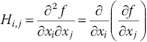
An important numerical value indicating the difficulty in predicting the real function with an interpolation model is the function curvature. The faster the function changes, the higher the curvature is and the more difficult it is to obtain a good prediction. The second criterion included in the toolbox is called Hessian and is based on this consideration. Starting from the available function samples, an interpolating Kriging model is generated. The approximated full model allows second derivative approximation with a central difference (second order of accuracy) to be calculated, as shown in Eq. (15.27).

The most important location is then evaluated as the point with the maximum mse belonging to a sphere centered on the point with the highest curvature and with radius equal to the distance from the nearest point already sampled. Finally the mse of the point found is compared with the global maximum of the mse divided by a custom scale and so the algorithm decides where to locate the next sample as the biggest between them. The Achilles heel of the second‐order derivative‐based criterion relates to points with non‐continuous first derivatives (cusps), for which the central difference returns very high values.
For n‐dimensional domain problems, a unique second‐derivative value is not available; there are different values when computed along different directions. In order to consider all the local second‐derivative values and not to be bounded to any frame of reference, an easy but reasonable way is as follows. The global problem is to find where a generic discrete function f exhibits the biggest curvature in space, with respect to any given direction. The Hessian matrix elements are defined as partial derivatives, as shown in Eq. (15.28a). If the second derivatives of f are all continuous, then the Hessian is a symmetric matrix (from the symmetry property of second derivatives, known as Schwarz’ or Clairaut’s theorem).
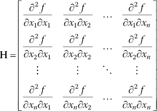
A finite difference approximation of the Hessian matrix is adopted. For the diagonal terms, which are pure second derivatives, the approximation with central difference presented in Eq. (15.27) is used, obtaining a second order of accuracy. The procedure of approximating the mixed second derivatives is based on central difference (second order of accuracy as well) and this is set out in Eq. (15.29). The ī and ![]() stand for the indices of the discrete domain, indicating the xi
and xj
coordinates of the analyzed point.
stand for the indices of the discrete domain, indicating the xi
and xj
coordinates of the analyzed point.

The Frobenius norm of the Hessian matrix, presented in Eq. (15.30), can then be used as numerical index of the function curvature. This value is not dependent on the frame of reference used, because the Frobenius norm is invariant under a unitary transformation, being a reference frame rotation.

For a multi‐outputs function, a criterion was developed in order to give priority to some outputs about the choice of the next sample location. If a very fast and efficient computation is needed, the user may prefer to focus on the main aerodynamic loads, such as lift, drag or pitching moment, and decide to have a more precise result for these, neglecting the others.
Applications
Two real cases are now considered in order to obtain validation for real data sets. The SACCON and the TCR test cases are outlined in Section 15.1.5.
In Figure 15.16 some aerodynamic coefficients of the UCAV SACCON are presented. The lift, drag and pitching moment coefficients with respect to the angle of attack are considered. The analysis conducted is one‐dimensional. Both of the sampling criteria available in the toolbox are used. The solutions give very good results, finding the sudden drop of the pitching moment with only 12 sample points for both methods (iteration number 10). For the maxima–minima criterion this is achieved because of the presence of a local maximum close to the non‐linearity in the pitching moment. For the second‐derivative‐based criterion, the pitching moment drop is found thanks to a high second derivative in the lift function at the same location, permitting further analyses to be made close to this non‐linearity. In these cases the mean relative errors of the pitching moment prediction compared to the target function are 2.40% with the maxima–minima criterion and 1.92% with the second‐derivative criterion. Both the prediction models predict the sudden and narrow aerodynamic non‐linearity that manifests itself as a pitching moment fall.


Figure 15.16 Comparing the results on the UCAV data after ten iterations and two initial samples at the extrema: (a) lift with local maxima–minima criterion; (b) pitching moment with local maxima–minima criterion; (c) lift with second derivative criterion; (d) pitching moment with second derivative criterion. From Cristofaro (2014).
The sampling methods are also applied to the TCR test case. In Figure 15.17, the coloured surface indicates the Kriging model prediction obtained with the sample points as circles. The diamonds show the discrete target function. The mean relative errors of the pitching moment predictions compared to the target function are 15.90% for the maxima–minima criterion and 13.12% for Hessian criterion. It can be seen that the two methods predict well the general trend of the function with only 14 samples (4 starting and 10 iterations). The relative error is relatively large, but only 14 points over 318 total points of the domain were analyzed (4.4% of the total required computation).

Figure 15.17 Comparing the results obtained with the two developed methods on the TCR data after 10 iterations (with 4 initial samples at the domain vertices). From Cristofaro (2014).
15.3.5 Data Fusion
The aerodynamic coefficients can be generally obtained using different sources. If more data sets are available, data fusion can combine them in order to obtain a more accurate model. If two data sets available, usually one can be considered low‐fidelity (lf, which is cheaper and usually more populated) and the other high‐fidelity (hf, which is more expensive and usually less populated). During the data fusion process the cheap samples provide information about the trend of the target function, while the expensive samples give quantitative information about the model. Two methods are used for data fusion:
-
Method of Da Ronch et al. (2011a
): A Kriging interpolation model
 is calculated from the samples of the cheap aerodynamic evaluations and it is evaluated at the locations at which expensive predictions are available,
  . The vector of the input parameters at the expensive samples, xi
, is then augmented by the evaluation of the Kriging function for the cheap samples:
. The vector of the input parameters at the expensive samples, xi
, is then augmented by the evaluation of the Kriging function for the cheap samples:  . A Kriging interpolation model is finally calculated for the augmented samples and the data‐fused evaluation is given by the evaluation of this function in the continuous vector
  .
. -
Method of Santini (
2009
): As in the previous algorithm, a Kriging interpolation model
 is calculated from the samples of the cheap aerodynamic evaluations.
This criterion is then based on an increment function
is calculated from the samples of the cheap aerodynamic evaluations.
This criterion is then based on an increment function  obtained with the interpolation of
  , where
  are the high‐fidelity sampled points. From this, the data fusion approximation is easily derived as
  .
.
The Da Ronch method has some problems with oscillations when dealing with the interpolation for a second‐order regression model because of the aligned nature of ![]() ; in the case of a linear low‐fidelity database, the resulting Kriging interpolation matrix is ill‐conditioned. For these reasons the function implemented tries to use this algorithm, but it does not always work; the user is advised to use the Santini method and to be very careful about the Da Ronch method.
; in the case of a linear low‐fidelity database, the resulting Kriging interpolation matrix is ill‐conditioned. For these reasons the function implemented tries to use this algorithm, but it does not always work; the user is advised to use the Santini method and to be very careful about the Da Ronch method.
Two similar data fusion cases are investigated using the Santini method. The high‐fidelity data are taken from results of the wind‐tunnel test data for a UCAV, as reported by Vallespin et al. (2011) and already used in the one‐dimensional validation in Section 15.3.4. The sample point choice is taken from the results of the previously described Hessian iterative sampling criterion. For the low‐fidelity data, in the first case a custom function presenting an initially linear behaviour and then a sudden drop is used. This function is slightly vertically shifted with respect to the high‐fidelity data. The second low‐fidelity case is taken from Vallespin et al. (2011) and represents the data from a CFD computation, involving solving RANS equations with a k‐ϵ turbulence model. This case is more realistic and represents a plausible real‐world scenario.
Figure 15.18a shows that, for a linear low‐fidelity data trend, the data fusion looks very similar to a linear interpolation of the high‐fidelity data. A small difference may appear close to the high curvature of the low‐fidelity function, for which the fused data try to represent the same bend. The second resulting fused data (Figure 15.18b) exhibits strong non‐linearity. The two data sets may appear similar but, because of the horizontal shifting of the curves, the fused data displays a high oscillation close to position of the non‐linearity. Theoretically we do not know this position precisely, and the low‐fidelity data information may be misleading. In conclusion, data fusion may bring some improvement, but the user is strongly advised to take a critical look at the results.

Figure 15.18 Data fusion applied to the UCAV wind tunnel high fidelity data with low two different fidelity data. From Cristofaro (2014).
Data fusion can be performed during the iterative sampling algorithm, obtaining a more accurate model of the function starting from the first iterations. The results after three iterations, with and without data fusion with the two previously described low‐fidelity databases, are presented in Figure 15.19. This shows that the prediction follows the low‐fidelity database. In the first case, the ease of the cheaply available results is that the resulting fused data are well approximated, but the non‐linearity is not found. The second case instead samples the non‐linear part, because of its presence in the cheap available results, but the overall function is a worse approximation. For this reason the user is advised to use data fusion during iterative sampling, but only for the first iterations, otherwise the low‐fidelity database might lead to inaccurate predictions.

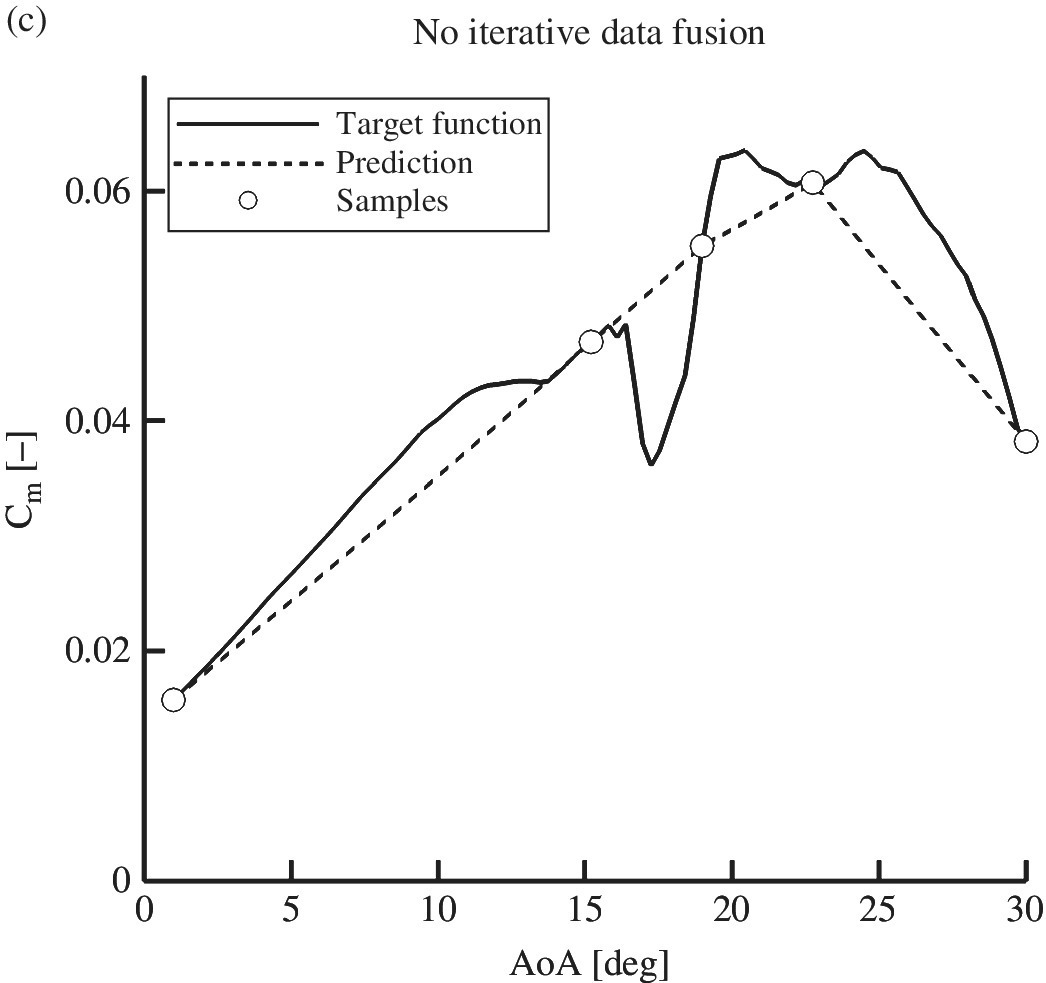
Figure 15.19 Iterative data fusion applied to the UCAV wind tunnel high‐fidelity data after three iterations for different low‐fidelity databases. From Cristofaro (2014).
15.3.6 Prediction of Dynamic Derivatives
Dynamic derivatives are calculated from observations of the responses of aerodynamic forces and moments to translational and rotational motions. Dynamic derivatives influence the aerodynamic damping of aircraft motions and are used to evaluate the aircraft response and the open‐loop stability, for example short‐period, Phugoid and Dutch roll modes.
A common wind‐tunnel testing technique for the prediction of dynamic derivatives relies on harmonic forced‐oscillation tests. After the decay of the initial transients, the nature of the aerodynamic loads becomes periodic. A time‐domain simulation of this problem requires significant computational effort. Several oscillatory cycles have to be simulated to obtain a harmonic aerodynamic response, and a time‐accurate solution requires a small time‐step increment to accurately capture the flow dynamics (Da Ronch et al. 2012; Mialon et al. 2011). Time‐domain calculations support a continuum of frequencies up to the frequency limits given by the temporal and spatial resolution, but dynamic derivatives are computed at the frequency of the applied sinusoidal motion.
It is therefore worthwhile to consider a frequency‐domain formulation to obtain a good estimate of the derivatives at reduced computational cost. These computational approaches, based on the harmonic balance (HB) and the linear frequency domain (LFD) methods, provide the ability to efficiently approximate the aerodynamics resulting from small, periodic and unsteady perturbations of the geometry of an aircraft configuration. By resolving only the frequencies of interest, the computational cost of dynamic derivatives is greatly reduced. Initially developed in the field of turbomachinery (Clark and Hall 2000; van der Weide et al. 2005), the HB and LFD methods have been subsequently used for the external aerodynamics of aircraft (Da Ronch et al. 2010, 2013). A large amount of research has been devoted to applications of the HB and the LFD technologies in a broad spectrum of engineering disciplines. There is the question of the influence of the approximations on the derivative predictions. A body of previous work (Da Ronch et al. 2013; Mialon et al. 2011) has looked at the adequacy of frequency‐domain methods for the rapid calculation of dynamic derivatives for use in flight dynamics analysis. Thorough investigations of the dependencies of dynamic derivatives on model parameters were performed for realistic flight conditions, and the limitations of the tabular aerodynamic models traditionally used by flight dynamicists were assessed (McCracken et al. 2012).
Method of Data Analysis
Two techniques to post‐process time‐domain sampled data obtained from unsteady time‐domain simulations are common. First, the transformation to the frequency domain is considered in order to gain insights into the frequency spectra of aerodynamic loads. To improve standard techniques, the method described in Da Ronch et al. (2012) can be adopted. Second, a regression‐based approach can be used. Here, the unknown vector of the approximate solution is obtained from the minimization of an appropriate function. More details can be found in Da Ronch et al. (2012, 2013).
Finally, note that an implementation of a highly accurate finite Fourier transform (FFT) is provided in the online ancillary material with this chapter. A comparison between the novel approach and standard FFT is performed for two test cases.
15.4 Time‐accurate CFD for Flight Simulations
CFD is becoming credible for the computation of aerodynamic time‐history effects. The flight dynamics of a manoeuvring aircraft could potentially be modelled by coupling the unsteady Reynolds‐averaged Navier–Stokes (URANS) equations and the dynamic equations governing the aircraft motion. The first attempts were limited to two‐dimensional test cases, while recently the coupled CFD‐flight dynamics of a full aircraft have been studied (Ghoreyshi et al. 2011a). However, the CFD‐flight dynamics simulations take substantially longer than when taking the forces and moments from look‐up tables, raising the open question of when the time history of the aerodynamics is required for flight dynamics analysis. A framework for investigating the limits, from flow unsteadiness, of aerodynamic tables is described in Ghoreyshi et al. (2011a). The particular demonstrations of this framework are made for a generic (and sharp leading‐edge) fighter performing time‐optimal manoeuvres with the aerodynamics given by the Euler equations.
The key functionality for the CFD solver is the ability to move the mesh. Two types of mesh movement are required. First, rigid rotation and translation are needed to follow the motion of the aircraft. Secondly, the control surfaces are deflecting throughout the motion, which can be achieved either by mesh deformation or a Chimera technique (Madrane et al. 2004).
Ghoreyshi et al. (2011a) compares the aerodynamic forces from the static and dynamic tabular models and the motion replay in the CFD framework. This is done for slow motions, where close agreement would be expected. The motions used are trimmed level flight, pull‐ups with constant and varying angles of attack, wingover and 90° turns. The comparisons test the CFD formulation of the manoeuvre replay, which is done in a time‐accurate fashion with control surface deflections.
A number of slow longitudinal and lateral manoeuvres were used to demonstrate that the tabular and replay aerodynamics agreed closely as expected. The cost of generating the static tables was the equivalent of 200 steady‐state calculations, and the simulation of each manoeuvre was possible in roughly one tenth of this for the cases shown. Then, a number of higher‐rate manoeuvres for a pull‐up were used to investigate the influence of dynamic and unsteady terms. At moderate rates, the addition of dynamic tabular terms brought the tabular predictions into agreement with the replay values. However, for a high angle of attack with high‐rate motion, the dynamic terms were not adequate to achieve agreement. A quasi‐steady calculation confirmed that the tabular prediction was correct, and so the disagreement was due to the influence of the history in the unsteady replay manoeuvre. This example shows the usefulness of the framework in investigating the limits of tabular aerodynamic models.
Results for slow‐, medium‐ and fast‐rate pull‐up manoeuvres are shown in Figure 15.20. The resulting lift coefficients are shown, together with the angle of attack time history. In the slow pull‐up manoeuvre, the angle of attack increases from 0° to 12° in 10 s. Since dynamic effects are expected to be small at these rates, tabular and replay values of the lift coefficient are in good agreement. For the medium‐rate manoeuvre, at low angles the static tabular predictions are close to the replay values, with significant differences at higher angles when vortical flow is present. The addition of the dynamic tabular terms gives good agreement with the replay values at low angles, and a much closer agreement at higher angles. Finally, in the fast manoeuvre a larger difference between the replay and static tabular predictions is evident at all angles. The addition of dynamic effects makes the tabular predictions close to replay values at lower angles of attack, but they cannot correct the discrepancy at higher angles when significant history effects due to vortical interactions are present. Note also the spikes from the replay solution, which are due to dynamic effects from the very rapid motion of the control surfaces.

Figure 15.20 Aerodynamic responses for pull‐up manoeuvres with tabular models and replay simulation.
From Ghoreyshi et al. (2011a).
Based on previous work (Da Ronch et al. 2012; Ghoreyshi et al. 2011a,b; 2010; Vallespin et al. 2012), tabular models are found to be inadequate to predict motions at critical conditions. Attempts to improve the traditional model have been made, the most notable being the studies presented in Da Ronch et al. (2011b, 2014; Ghoreyshi et al. 2013).
15.4.1 Advanced Mathematical Models
The prediction of unsteady non‐linear flow conditions is an important part of aircraft design. The ability to predict the aerodynamic loads with some realism within the aerodynamic design cycle can accelerate industrial design processes and avoid costly design changes. Because of the need for short computing times, industrial analysis procedures often rely on low‐fidelity numerical aerodynamic methods. However, a large body of work on virtual flight simulation has revealed that the traditional model, based on stability derivatives, is inadequate for modelling unsteady aerodynamic effects for modern manoeuvring aircraft. In response to the need to improve the fidelity of simulations while keeping the computational costs low, more sophisticated models of the aerodynamics have been proposed.
Creating a full‐order model for stability and control (S&C) analysis is a computationally expensive approach because such a model needs a large number of coupled computations for different values of motion frequency and amplitude. An alternative approach to creating the full‐order model is to develop a reduced‐order model (ROM) that approximates CFD results by extracting information from a limited number of full‐order simulations. Ideally, the specified ROM can predict aircraft responses over a wide range of amplitudes and frequencies within a few seconds, without the need to re‐run CFD simulations. Recent efforts on the development of ROMs can be classified into two types: time‐domain and frequency‐domain approaches. The frequency‐domain models are obtained from matching transfer functions computed from the measured input–output data. Examples of frequency‐domain ROMs are the indicial response method of Ballhaus and Goorjian (1978) and a frequency‐domain approach based on proper orthogonal decomposition by Hall et al. (1999). Some examples of time‐domain ROMs include the Volterra theory, radial basis functions, and state‐space modeling (Goman and Khrabov 1992). These ROM techniques have been used extensively for flutter prediction, limit cycle oscillation, and gust‐response modelling, but their application to S&C is still new. Also, only a few studies have been conducted for reduced‐order modelling of aircraft configurations, mostly limited to the subsonic flow regime. Two techniques, one based on the Volterra series and one on non‐linear indicial functions, are reviewed in this section.
Denote as y the output quantity that is of interest in the aerodynamic simulation, and as x the input parameter that influences y. For example, y may refer to the aerodynamic pitch moment, and x to the angle of attack. The reduced‐order models try to define a simple yet non‐linear relationship that fits the dependency of y on x.
Volterra Series
Following the developments of the Volterra theory (Volterra 1930), the output of a continuous‐time, casual, time‐invariant, fading memory system in response to the input vector x(t) can be modeled using the pth‐order Volterra series shown in Eq. 15.31.
where ℍ represents the multi‐input Volterra operator. For example, the output response of a multi‐input Volterra series up to second order is formulated in Eq. 15.32.

Note that the superscripts in Eq. 15.32 identify to which inputs the kernel corresponds; for example, the second‐order kernel ![]() correlates the inputs
correlates the inputs ![]() and
and ![]() . Note that the second‐and higher‐order kernels are symmetric with respect to the arguments
. Note that the second‐and higher‐order kernels are symmetric with respect to the arguments ![]() . The accurate determination of the Volterra kernels is critical for the generation of an efficient, robust and non‐linear model. Techniques to identify the Volterra kernels from CFD calculations are discussed at the end of this section.
. The accurate determination of the Volterra kernels is critical for the generation of an efficient, robust and non‐linear model. Techniques to identify the Volterra kernels from CFD calculations are discussed at the end of this section.
Non‐linear Indicial Functions
We start with a linear indicial function defined by the relationship in Eq. 15.33.
where A represents the unit response, or indicial function, of the system. For a linear system, H 1 is the impulse response function and H 1(t) = dA(t)/dt applies. The indicial response functions are used as a fundamental approach to represent the unsteady aerodynamic loads. For non‐linear aerodynamic responses due to motions starting from different Mach numbers, the dependencies on the angle of attack and Mach number are added to the indicial functions in Eq. 15.34.
where M denotes the freestream Mach number. The response function due to pitch rate Cmq (α, M) can be estimated using a time‐dependent interpolation scheme from the observed responses. A possible technique is based on the surrogate modelling approach, as discussed in Section 15.3.2.
System Identification and Results
The generation of reduced models is done by post‐processing the output time history in response to a prescribed input time history. The choice of the most appropriate input signals is somewhat dependent on the specific applications of the reduced model, and a globally valid approach seems not to exist. As reported in Ghoreyshi et al. (2013), common input time histories, denoted as training manoeuvres, are the linear chirp, spiral and Schroeder functions. These training manoeuvres are shown in Figure 15.21.
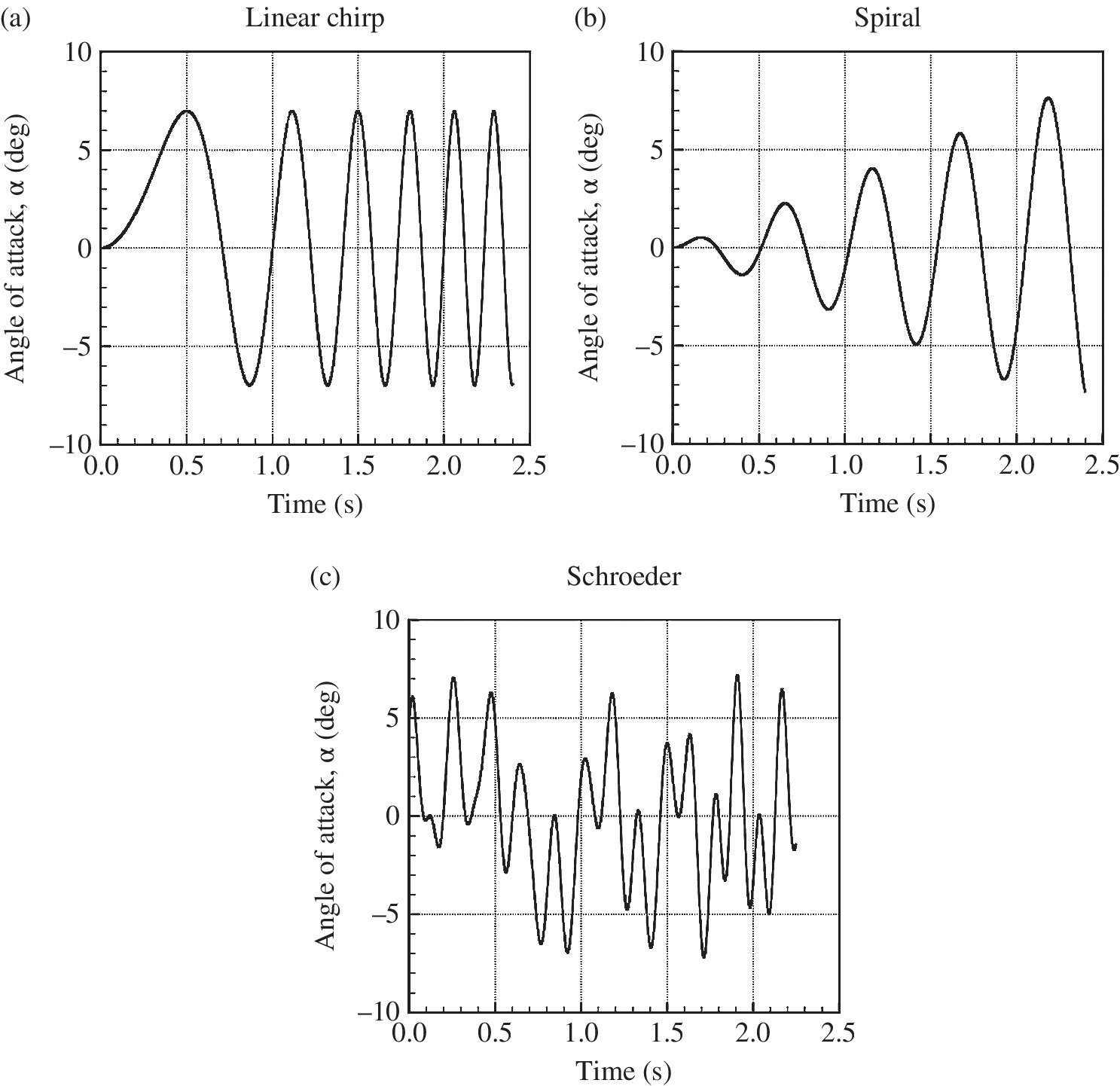
Figure 15.21 Training manoeuvres used to generate Volterra and indicial models.
From Ghoreyshi et al. (2013).
The test case of Ghoreyshi et al. (2013) is the X‐31 aircraft, a super‐manoeuvrable fighter with a canard wing and a double delta wing. The complex flow features around the X‐31 aircraft are shown in Figure 15.22.

Figure 15.22 X‐31 vortical flows using SARC‐DDES turbulence model. The conditions are M∞ = 0.18 and Re = 2 × 10⁶.
From Ghoreyshi et al. (2013).
The Volterra ROM predictions based on spiral and chirp training manoeuvres are compared with the time‐accurate solution data in Figure 15.23. There is good agreement with CFD data for a ROM identified from spiral data, but the ROM identified from chirp data does not match well, in particular around the maximum and minimum angles of attack. The instantaneous frequency in the chirp manoeuvre varies with time, and hence it might not have sufficient information to identify the Volterra kernels corresponding to a swept‐amplitude motion at constant frequency. However, the ROM based on chirp data could be used for predicting aerodynamic responses from pitch oscillations at many other frequencies (those covered by the simulation of the chirp training manoeuvre), but the ROM based on the spiral is possibly valid for motions at a fixed reduced frequency.

Figure 15.23 Volterra reduced–order modeling using spiral and chirp training maneuvers.
From Ghoreyshi et al. (2013).
The full‐order model is compared with the predictions from a linear ROM of the target manoeuvre in Figure 15.24a. The linear ROM fails to accurately predict the pitching moment values at all angles of attack. The functions of ![]() vary largely with angle of attack at transonic speeds, and thus a linear ROM cannot predict these effects.
vary largely with angle of attack at transonic speeds, and thus a linear ROM cannot predict these effects.
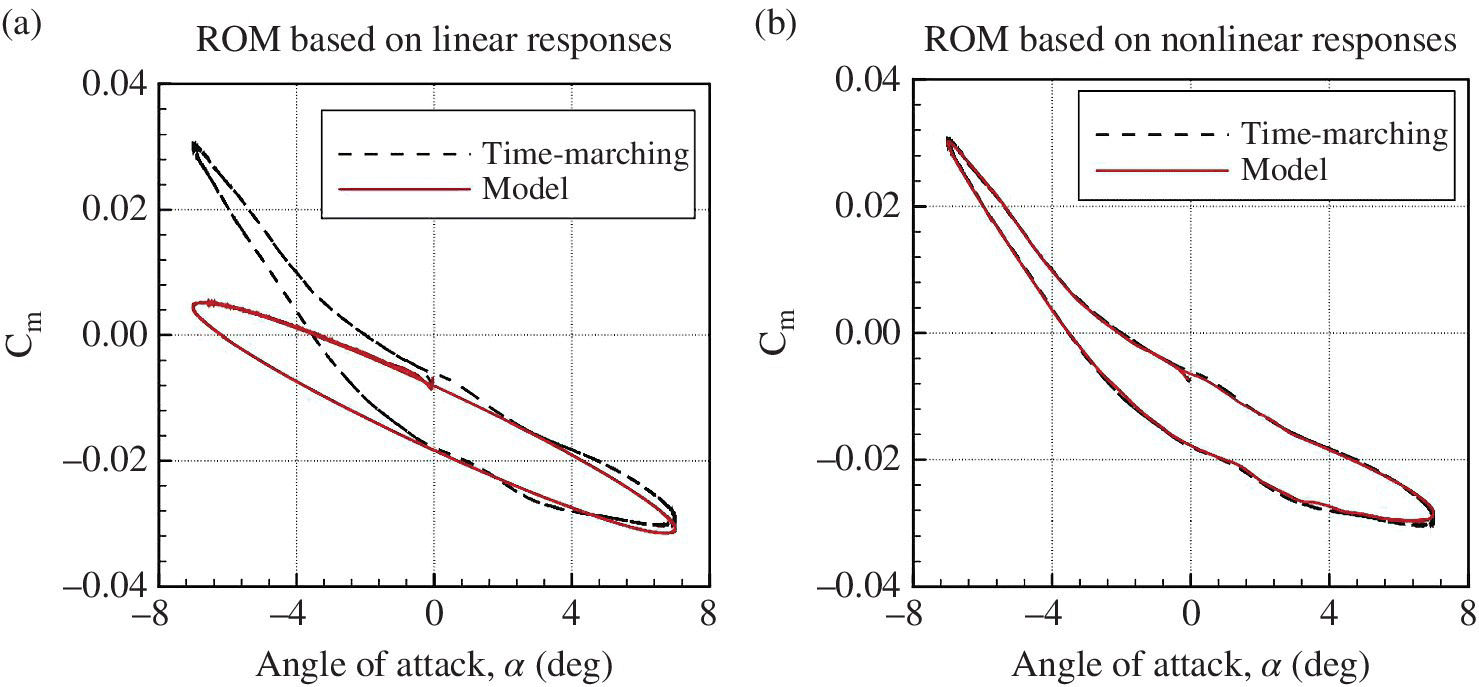
Figure 15.24 Indicial functions reduced‐order modeling using spiral and chirp training maneuvers.
From Ghoreyshi et al. (2013).
A non‐linear ROM was then created with Eq. 15.34 and, using a linear interpolation scheme, the prediction of the target manoeuvre was evaluated. Figure 15.24b shows that the non‐linear ROM predictions agree very well with full‐order simulation values. Note that such a non‐linear ROM may be used for computing the pitching moment responses from many other motions with different amplitudes and frequencies.
Cost of Generating the ROM
The objective of Ghoreyshi et al. (2013) was to generate cost‐effective reduced‐order models capable of predicting aerodynamic loads of an aircraft pitching within the frequency/amplitude/Mach space of interest. This work formed the basis for further studies of flight dynamics, where forces and moments were given by these models. Each reduced‐order model used carries a different computational cost and is based on various simplifying assumptions pertaining to the flow physics. For example, the generation of linear indicial functions is relatively inexpensive, but the model is limited to small‐amplitude motions at the fixed Mach number for which functions were calculated. A first‐order linear Volterra model has the same limitations. The non‐linear indicial functions include responses to different angles of attack and could be used for predicting responses to arbitrary motions at a fixed Mach number, but they have relatively high computational costs compared with a linear model. A Volterra model with second‐ and higher‐order kernels has the non‐linear dependencies of aerodynamic loads with amplitude. However, the suitability of the model for predicting responses to new motions depends on the type of training manoeuvre used to estimate kernels. A model that includes Mach number effects significantly increases the computational cost because it requires many calculations for each combination of angle of attack and Mach number.
15.5 Conclusions
The inadequacy and shortcomings of current industrial design procedures is apparent when confronted with the stringent environmental constraints demanded for controlling the impact of aviation on the environment and communities around airports. In need of fast turnaround times, industrial procedures are based on low‐fidelity empirical and linear approximations. Having recognised the urgency of increasing the realism of predictions for better designs and reducing the time to bring new aircraft to market, this chapter has presented state‐of‐the‐art methods for virtual flight simulation. The development of a unified approach, capable of assisting the aircraft designer to investigate unconventional configurations and identify critical design features that may jeopardise the aircraft programme if discovered late in the design process, is instrumental to meeting the ambitious goals of EU and USA.
References
- Ballhaus WF and Goorjian PM 1978 Computation of unsteady transonic flow by the indicial method. AIAA Journal 16(2), 117–124. doi: 10.2514/3.60868.
- Beyers ME 1995 Interpretation of experimental high‐alpha aerodynamics – implication for flight prediction. Journal of Aircraft 32(2), 247–261.
- Bryan GH 1911 Stability in Aviation. MacMillan, London.
- Chambers JR and Hall RM 2004 Historical review of uncommanded lateral‐directional motions at transonic conditions. Journal of Aircraft 41, 436–447.
- Clark WS and Hall KC 2000 A time–linearized Navier–Stokes analysis of stall flutter. Journal of Turbomachinery 122(3), 467–476. doi: 10.1115/1.1303073.
- Cressie NAC 1991 Statistics for Spatial Data. Wiley.
- Cristofaro M 2014 Elements of Computational Flight Dynamics for a Complete Aircraft Masters thesis, Politecnico di Torino, Italy and University of Southampton, U.K.
- Cristofaro M, Wang Y and Da Ronch A 2014 Towards computational flight dynamics of a passenger jet aircraft ICAS International Council of Aeronautical Sciences Conference, vol. 0462, St Petersburg, Russia.
- Da Ronch A 2012 On the Calculation of Dynamic Derivatives using Computational Fluid Dynamics. PhD Thesis, University of Liverpool, Liverpool, UK.
- Da Ronch A, Ghoreyshi M and Badcock KJ 2011a On the generation of flight dynamics aerodynamic tables by computational fluid dynamics. Progress in Aerospace Sciences 47(8), 597–620.
- Da Ronch A, Ghoreyshi M, Badcock KJ, Görtz S, Widhalm M, Dwight RP and Campobasso MS 2010 Linear frequency domain and harmonic balance predictions of dynamic derivatives 28th AIAA Applied Aerodynamic Conference Chicago, IL. AIAA Paper 2010‐4699.
- Da Ronch A, McCracken A, Badcock KJ, Ghoreyshi M and Cummings RM 2011b Modeling of unsteady aerodynamic loads AIAA Atmospheric Flight Mechanics Conference, Portland, OR. AIAA Paper 2011–6524, doi: 10.2514/6.2011‐6524.
- Da Ronch A, McCracken AJ, Badcock KJ, Widhalm M and Campobasso MS 2013 Linear frequency domain and harmonic balance predictions of dynamic derivatives. Journal of Aircraft 50(3), 694–707. doi: 10.2514/1.C031674.
- Da Ronch A, McCracken AJ, Tantaroudas ND, Badcock KJ, Hesse H and Palacios R 2014 Assessing the impact of aerodynamic modelling on manoeuvring aircraft AIAA SciTech 2014, AIAA Atmospheric Flight Mechanics Conference. AIAA Paper 2014‐0732. doi: 10.2514/6.2014‐0732.
- Da Ronch A, Vallespin D, Ghoreyshi M and Badcock KJ 2012 Evaluation of dynamic derivatives using computational fluid dynamics. AIAA Journal 50(2), 470–484. doi: 10.2514/1.J051304.
- Forsythe JR, Fremaux CM and Hall RM 2006 Calculation of static and dynamic stability derivatives of the F/A‐18e in abrupt wing stall using RANS and DES. In: Computational Fluid Dynamics 2004 (eds. Groth C and Zingg DW). Springer, pp. 537–542. doi: 10.1007/3‐540‐31801‐1_76.
- Ghoreyshi M, Badcock KJ and Woodgate MA 2009 Accelerating the numerical generation of aerodynamic models for flight simulation 47th AIAA Aerospace Sciences Meeting including the New Horizons Forum and Aerospace Exposition, Orlando, Florida.
- Ghoreyshi M, Badcock KJ, Da Ronch A, Marques A, Swift A and Ames N 2011a Framework for establishing limits of tabular aerodynamic models for flight dynamics analysis. Journal of Aircraft 48(1), 42–55. doi: 10.2514/1.C001003.
- Ghoreyshi M, Badcock KJ, Da Ronch A, Vallespin D and Rizzi A 2011b Automated CFD analysis for the investigation of flight handling qualities. Mathematical Modelling of Natural Phenomena 6(3), 166–188.
- Ghoreyshi M, Cummings RM, Da Ronch A and Badcock KJ 2013 Transonic aerodynamic loads modeling of X–31 aircraft pitching motions. AIAA Journal 51(10), 2447–2464. doi: 10.2514/1.J052309.
- Ghoreyshi M, Vallespin D, Da Ronch A, Badcock KJ, J. V and Hitzel S 2010 Comparisons of computational fluid dynamics solutions of static and manoeuvring fighter aircraft with flight test data AIAA Atmospheric Flight Mechanics Conference, Toronto, Ontario.
- Giunta AA, Wojtkiewicz SFJ and Eldred MS 2003 Overview of modern design of experiments methods for computational simulations 41st Aerospace Sciences Meeting and Exhibit. AIAA Paper 2003–649.
- Goman MG and Khrabov AN 1992 State–space representation of aerodynamic characteristics of an aircraft at high angles of attack Astrodynamics Conference. AIAA Paper 1992‐4651.
- Greenberg H 1951 A survey of methods for determining stability parameters of an airplane from dynamic flight measurements. Technical report TN‐2340, NACA.
- Hall KC, Thomas JP and Dowell EH 1999 Reduced–order modelling of unsteady small–disturbance using a frequency–domain proper orthogonal decomposition technique 37th Aerospace Sciences Meeting and Exhibit. AIAA Paper 1999‐655.
- Hastings WK 1970 Monte Carlo sampling methods using Markov chains and their applications. Biometrikam 57, 97–109.
- Isaaks EH and Srivastava RM 1989 Applied Geostatistics. Oxford University Press.
- Jones DR, Schonlau M and Welch WJ 1998 Efficient global optimization of expensive black‐box functions. Journal of Global Optimization 13(4), 455–492.
- Loeser T, Vicroy D and Schuette A 2010 Saccon static wind tunnel tests at Dnw–Nwb and 14 × 22 NASA LARC 28th AIAA Applied Aerodynamics Conference. AIAA Paper 2010–4393.
- Mackman TJ, Allen CB, Ghoreyshi M and Badcock KJ 2013 Comparison of adaptive sampling methods for generation of surrogate aerodynamic models. AIAA Journal 51(4), 797–808.
- Madrane A, Raichle A and Stürmer A 2004 Parallel implementation of a dynamic overset unstructured grid approach ECCOMAS Conference, Jyväskylä, Finland.
- Mason WH, Knill DL, Giunta AA, Grossman B, T. WL and T. HR 1998 Getting the full benefits of CFD in conceptual design 16th AIAA Applied Aerodynamics Conference, Albuquerque, NM. AIAA Paper 1998–2513
- McCracken A, Akram U, Da Ronch A and Badcock KJ 2012 Requirements for computer generated aerodynamic models for aircraft stability and control analysis 5th Symposium on Integrating CFD and Experiments in Aerodynamics, Tokyo, JP, 3–5 October 2012.
- McDaniel DR, Cummings RM, Bergeron K, Morton SA and Dean JP 2010 Comparisons of computational fluid dynamics solutions of static and manoeuvring fighter aircraft with flight test data. Journal of Aerospace Engineering 223, 323–340.
- Mialon B, Khabrov A, Ben Khalil S, Hebner A, Da Ronch A, Badcock K, Cavagna L, Eliasson P, Zhang M, Ricci S, Jouhaud J, Roge G, Hitzel S and Lahuta M 2011 Validation of numerical prediction of dynamic derivatives: The DLR‐F12 and the transcruiser test cases. Progress in Aerospace Sciences 47, 674–694.
- Mialon B, Khrabov A, Ricci S, Eliasson P, Huebner A and Larsson R 2010 Benchmarking the prediction of dynamic derivatives: Wind tunnel tests, validation, acceleration methods Special session AIAA AFM conference, Toronto.
- Mueller T 1985 The influence of laminar separation and transition on low Reynolds number airfoil hysteresis. Journal of Aircraft 22(9), 763–770.
- Napolitano MR 2011 Aircraft Dynamics: From Modeling to Simulation. Wiley.
- Rizzi A, Eliasson P, Goetzendorf‐Grabowski T, Vos JB, Mengmeng Z and Richardson TS 2011 Design of a canard configured transcruiser using Ceasiom. Progress in Aerospace Sciences 47(8), 695–705.
- Rogers SE, Aftomis MJ, Pandya SA, Chaderjian NM, Tejnil ET and Ahmad JU 2003 Automated CFD parameter studies on distributed parallel computers 16th AIAA Computational Fluid Dynamics Conference, Orlando, Florida, 23–26 June 2003. AIAA Paper 2003‐4229.
- Santini D 2009 Adaptive Fidelity Aero Data Generation Masters thesis Politecnico di Milano, Italy and Royal Institute of Technology, Stockholm, Sweden.
- Scharl J, Mavris DN and Burdun IY 2000 Use of flight simulation in early design: Formulation and application of the virtual testing and evaluation methodology 2000 World Aviation Conference, San Diego, CA, pp. 436–447.
- Shewry MC and Wynn HP 1987 Maximum entropy sampling. Journal of Applied Statistics 14(2), 165–170.
- Snyder J 1990 CFD needs in conceptual design Aircraft Design, Systems and Operations Conference, Aircraft Design and Operations Meetings. AIAA Paper 1990‐3209.
- Vallespin D July 2012 Development of a Process and Toolset to Study UCAV Flight Mechanics using Computational Fluid Dynamics. PhD Thesis, University of Liverpool, Liverpool, UK.
- Vallespin D, Badcock KJ, Da Ronch A, White M, Perfect P and Ghoreyshi M 2012 Computational fluid dynamics framework for aerodynamic model assessment. Progress in Aerospace Sciences 52, 2–18. doi: 10.1016/j.paerosci.2011.12.004.
- Vallespin D, Da Ronch A, Badcock KJ and Boelens O 2011 Vortical flow prediction validation for an unmanned combat air vehicle model. Journal of Aircraft 48(6), 1948–1959.
- Vallespin D, Ghoreyshi M and Badcock KJ 2010 Assessment of the limits of tabular aerodynamic models for flight dynamics analysis using the SACCON UCAV configuration RAeS Aerodynamics Conference, Bristol.
- van der Weide E, Gopinath AK and Jameson A 2005 Turbomachinery applications with the time spectral method 35th AIAA Fluid Dynamics Conference and Exhibit. AIAA Paper 2005–4905.
- Venkatakrishnan L, Sundaram S and Viswanath PR 2006 Hysteresis and broad flow features on a swept wing at high lift. Journal of Aircraft 43(4), 1036–1043.
- Volterra V 1930 Theory of Functionals. Blackie.
- Williams JE and Vukelich SR 1979 The USAF stability and control digital DATCOM. Technical report AFFDL–TR–79–3032, McDonnell Douglas Astronautics Company.
- Woodson SH, Green BE, Chung JJ, Grove DV, Parikh PC and Forsythe JR 2005 Understanding abrupt wing stall with computational fluid dynamics. Journal of Aircraft 42(3), 578–585.
- Zhang M, Tomac M, Wang C and Rizzi A 2013 Variable fidelity methods and surrogate modeling of critical loads on X‐31 aircraft 51st AIAA Aerospace Sciences Meeting including the New Horizons Forum and Aerospace Exposition, Grapevine, Texas, USA, vol. 1081.