
10
Framework for the Optimisation of a Helicopter Rotor Blade with an Approximate BERP Tip: Numerical Methods and Application
Catherine S. Johnson, Mark Woodgate and George N. Barakos
School of Engineering, University of Liverpool, UK
School of Engineering, University of Glasgow, UK
10.1 Introduction
10.1.1 BERP Blade
The BERP blade has a ‘paddle‐shaped’ tip due to a forward displacement of the planform (creating a notch), followed by sweep, as shown in Figure 10.1. It is a benchmark design because of its improved performance in forward flight, winning it a world speed record for helicopter flight (Perry et al. 1998). Some CFD analysis was carried out for this blade in order to find the specific reasons for its improved performance, and to analyse what happens in the flowfield around it (Brocklehurst and Duque 1990). However, at the time, computational power was limited and today, higher fidelity CFD methods are available. The aim of this chapter is to apply CFD and optimisation methods to investigate if further performance enhancements can be obtained by fine‐tuning specific features of the BERP tip. At the same time, the methods outlined in Chapter 9 are applied. A brief history of the BERP blade development is presented below.

Figure 10.1 Definition of the parameters of the BERP‐like blade.
The BERP tip was designed for high‐speed forward flight without compromising hover performance (Harrison et al. 2008). The problem associated with the fast forward flight regime, is that the effects of compressibility, such as transonic flow and shockwaves, become significant, especially on the advancing blade. Typically, thin aerofoils are used but these tend to stall more easily at the high angles of attack that occur on the retreating side. The first step in the design of the BERP was the aerofoil selection. The aerofoils were selected such that thinner sections could be used to enable higher forward flight speeds. Camber was introduced to improve the stall capability of the blade on the retreating side, and the increased pitching moments were alleviated by having a reflexed aerofoil inboards. The resulting blade is reported to behave well in terms of control requirements and twist loads (Robinson and Brocklehurst 2008).
The planform was then optimised to reduce high‐Mach‐number effects by first sweeping the tip of the blade back. This moved the aerodynamic centre of the swept part backwards, causing control problems in the pitch axis. To counteract this, the swept part was translated forward, which introduced a notch on the leading edge of the blade. The notch corners were smoothed to avoid flow separation. A ‘delta’ tip was also incorporated, so that a stable vortex formed at higher angles of attack on the retreating side to delay stall (Brocklehurst and Duque 1990).
One of the characteristics of the blade is that blade stall occurs first inboards of the notch and does not spread outwards. This is because at high angles of attack, such as at the retreating side, the vortex formed travels around the leading edge and the flow over the swept part remains attached. The BERP blade shows similar performance to a standard rotor blade in low‐speed flight, but superior performance in forward flight due to the absence of drag rise and flow separation (Brocklehurst and Duque 1990). In hover, the figure of merit (FM) was improved due to the minimisation of blade area and, overall, there were no penalties in hover performance. At high speeds, blade vibration was also reduced, as were control loads for manoeuvres (Brocklehurst and Duque 1990).
The next sections describe how a BERP‐like rotor blade tip can be optimised for improved performance given certain constraints. The same method can be applied to UAVs to improve any aspect of their performance within any given constraints.
10.2 Numerical Methods
Fully analysing a rotor using time‐marching CFD methods, even when parallel computing is used, can take hours of clock time. Another technique that can be used to obtain the performance of the rotors to the same accuracy (provided a sufficient number of modes is used), is the harmonic balance (HB) method (Woodgate and Barakos 2009).
With HB, the time taken to perform the same calculation can be an order of magnitude less than the time taken using time‐marching. This greatly improves the efficiency of the optimisation process, making it a more usable technique for rotor design. The number of snapshots (N S ) obtained is given as
where N H is the number of modes. Here, four modes were used, resulting in nine snapshots; in other words, every 40°. Since this is a four‐bladed rotor, it results in a blade snapshot at every 10° of azimuth. This is because blade 1 of the rotor will be captured at 40, 80, 120, 160, 200, 240, 280, 320 and 360° of azimuth and since blade 2 is 90° away from blade 1, in the same snapshots, blade 2 will be at 130, 170, 210, 250, 290, 330, 370 (which is 10), 410 (which is 50) and 450 (which is 90) degrees. Similarly for blades 3 and 4, there will be a shift of 10° from the previous blade, resulting in a snapshot at every 10° of azimuth. The method has been shown to give results of similar accuracy to time‐marching methods in Woodgate and Barakos (2009). A brief summary of the method is given here.
The HB method uses the governing (Navier–Stokes) equations in the frequency domain. Equation (10.2) represents the governing equations, where Q(t) is the matrix of each solution variable such as pressure, density and velocity components, and R(t) is the residual for each of these variables; these are assumed to be periodic.

Then, expressing the solution as a Fourier series with a fixed number of modes, N H :

where ω is the rotational speed of the rotor. A Fourier transform of Eq. (10.5) gives

This gives a system of N
T
equations, where ![]() , for the Fourier series coefficients:
, for the Fourier series coefficients:
This is expressed in matrix form as:
where M is an ![]() matrix.
matrix.
R(t) is a function of Q(t) and it is non‐linear. Therefore each coefficient ![]() depends on all the coefficients
depends on all the coefficients ![]() and hence must be solved iteratively. There are a number of ways that this can be carried out.
and hence must be solved iteratively. There are a number of ways that this can be carried out.
In the pseudo‐spectral method, the equations are transformed back to the time domain and the period is split into N T equal discrete time intervals or snapshots, represented as Q hb and R hb . Then Eq. (10.12) is decomposed to form,
where ![]() , and E is a transformation matrix transforming
, and E is a transformation matrix transforming ![]() and
and ![]() to Q
hb
and R
hb
. The diagonal of D is zero and pseudo time‐marching can then be applied to the HB equation
to Q
hb
and R
hb
. The diagonal of D is zero and pseudo time‐marching can then be applied to the HB equation
However, other methods exist that use less memory, which can be a limiting factor in the use of the HB method. More details are given in Woodgate and Barakos (2009) and Jang et al. (2012).
The helicopter multi‐block method is a parallel CFD code that is used routinely for the analysis of rotors (Steijl et al. 2005). The method was validated for popular rotor cases like the Caradonna and Tung (1981) and the ONERA 7A and 7 AD rotors (Steijl and Barakos 2008). These efforts are described in the literature (Steijl et al. 2006).
In this study, the turbulence model used was the ![]() two‐equation model. The calculations were run with a third‐order spatial scheme, and the unsteady Reynolds averaged Navier–Stokes (URANS) equations. No wake model was used. Multiblock structured grids were used, the details of which are given in Section 10.5. The computations were all trimmed to give the same thrust‐to‐rotor solidity values. Geometric solidity was used and calculated as follows:
two‐equation model. The calculations were run with a third‐order spatial scheme, and the unsteady Reynolds averaged Navier–Stokes (URANS) equations. No wake model was used. Multiblock structured grids were used, the details of which are given in Section 10.5. The computations were all trimmed to give the same thrust‐to‐rotor solidity values. Geometric solidity was used and calculated as follows:

where N b is the number of blades and A b is the area of the blade, calculated by integrating the chord along the radius, R. No aeroelastic or structural model was used and the blades were treated as rigid blades. Once an initial solution was obtained, it was possible to use this solution as a starting point for another variation of the BERP‐like tip.
10.3 Optimisation Method
As seen in Chapter 9, there has been substantial research and interest in the use of genetic algorithms (GAs) in the optimisation of rotors. However, application and development in the past has mostly occurred in the design of compressors, turbines or electric rotors, where the ratio of the blade size to the actual rotor is quite low (Mengistu and Ghaly 2008; Samad and Kim 2008; Zhao et al. 2008). In the case of helicopter and other rotorcraft rotors, gradient‐based methods have been popular, because they have a lower demand for computational effort, time and cost. Non‐gradient based methods should be able to identify global optima, but the high computational effort involved has rendered these methods impractical for rotor optimisation.
Nevertheless, there are a number of methods that could reduce the computational effort in terms of CPU time as well as storage and, with the advances made in computing power, the use of these methods in rotor optimisation is becoming more feasible. The use of metamodels or surrogate models can reduce the calculation time and is expected to counteract the extra optimisation time required to apply non‐gradient based optimisation techniques whilst still maintaining global optimisation. Figure 10.2 is a map of the stages involved in the optimisation. It is an aposteriori‐type method according to Régnier et al. (2005). The work described here aims to demonstrate a framework, allowing different aspects of rotors and fuselages to be aerodynamically optimised given an existing design as a starting point. For real helicopter rotors, the initial designs would already be near optimum and the aim is to capture the aerodynamic effects of any design changes and adjust the variables of the design to find an optimum that will lead to better rotor performance.

Figure 10.2 Map of the processes involved in the optimisation of rotors.
10.3.1 Optimisation Framework
To improve the efficiency a non‐gradient‐based method, the high‐fidelity solver is decoupled from the optimisation loop. It is, however, available to the optimiser through a database. Therefore, the first step in the process is to create a database or population of designs. It is important for the design parameters to be clearly defined, along with the boundaries of the database and the constraints. These must be user‐defined and are based on experience and the requirements of the optimisation case. A parameterisation technique must be created if it does not already exist for the case. The boundaries of these parameters are then set, based on engineering expertise of the problem and the case in question. Once these have been determined, a sampling method is used to generate a number of design points to create the database or design space using the high‐fidelity solver. For each case, the geometry is modified and run using the high‐fidelity solver.
The next step is to determine the performance parameters that capture the objectives of the optimisation and to then combine these into a single value that the optimiser can use to determine the overall performance of an individual design. This again is dependent on the experience of the user, but is also guided by the performance of the designs in the database and further supported by other optimisation criteria such as the Pareto front method (Daskilewicz and German 2012; Oyama et al. 2010).
The optimiser now uses the database (which represents the design space) to determine the performance of a design point. However, it may need to evaluate the performance of a design point that may not exist in the database and therefore the CFD solver will have to be used. This would incur a large computational cost and time, because such requirements tend to occur often. To overcome this, a metamodel is used to predict the performance of unknown design points based on the performance of the existing points in the database by some interpolation technique. The accuracy or the tolerance value of the error in these predictions is what determines the resolution of the design parameter values in the database. The metamodel can be validated using a small number of additional design points obtained using the high‐fidelity solver. A selection of different metamodels were tested in our work, including artificial neural networks (ANNs), kriging, polynomial fits and proper orthogonal decomposition (POD). Of these, the first two were the most successful in terms of accuracy and efficiency. The optimiser can then employ the predictions of the metamodel to obtain the performance of new designs quickly. After a number of iterations, the designs are expected to converge to an optimum or a cluster of optimal designs. The optimiser is able to exercise constraints specified by the user. The final new design is then validated using the high‐fidelity solver.
The sampling method used was a full factorial method due to the small number of points in the database. However, for a larger‐scale optimisation project with more design parameters, such as the optimisation of a multi‐segment fixed wing planform, other sampling methods may provide better efficiency without loss of accuracy. Such methods include the fractional‐factorial method and Latin hypercube sampling (LHS), amongst others.
The rest of this section describes each stage of the optimisation in more detail and the following sections present an application example and results.
10.3.2 Sampling the Design Space
There are a number of ways that the database can be populated (Simpson et al. 2001). In the example used here, the full‐factorial method was used. Short descriptions of the fractional factorial and the LHS methods are also given here.
The full factorial method analyses all other variables for each design variable. Therefore it has the highest number of design points. The fractional factorial method uses every other point of the full factorial method; in other words, it is a sparser version of the full factorial database. If the area of the design space where the optimum is expected to be found is known, then the points selected using this method can be such that there is a higher concentration of design points in that area; that is, with those parameter values. This can be found by repeating the optimisation a number of times with additional points in the database each time, a process also known as ‘adaptive sampling’ or ‘updating’ (Forrester and Keane 2009).
The LHS method attempts to use a design parameter value only once or as few times as possible in populating the database. So, for example, if there are two parameters with equal number of design parameters, the LHS will select the design points along the diagonal line (or on a hyperplane for larger numbers of parameters) of the database. If there are more variables for one design parameter than another, then a random additional point is created for the component that has fewer variables. Sometimes it is necessary to also include the parameter values of the boundary of the database for enhanced accuracy.
The more points in the database, the more accurate the metamodel predictions will be. This means that the full factorial method will always produce the most accurate results. However, for cases where the computation time and cost of obtaining the performance of each design point is high, it is important to reduce the number of such calculations by selecting as few points as possible, as in the case of fractional factorial and LHS methods. These methods can produce good results if the points are selected carefully and if some additional points on the boundary of the database are included. Cameron et al. (2011) used an automated adaptive sampling method to optimise laminar flow aerofoils. In his method, the Pareto front was updated after a set number of generations and the mean square error of the kriging metamodel was used to calculate the probability that a new sample added at any given point would dominate members of the existing Pareto front. This process was automated in the genetic algorithm used, NSGAII (Cameron et al. 2011), and repeated until a set sample size was obtained. Forrester et al. (2008) also describe an optimal LHS method based on adaptive sampling.
10.3.3 Objective Function
The objective function determines the outcome of the optimisation. An ideal objective function should be, according to Tan et al. (2002):
- complete, so that all aspects of the decision problem are presented
- operational – it can be used in a meaningful manner
- decomposable, if disaggregation of the function is required
- non‐redundant, so that no aspect of the decision is considered twice
- minimal, so that the function considers the minimum required for a decision.
In line with these properties, the objective function is presented as the summation of weighted components that quantify the objectives. The actual values of each component that makes up the objective function may vary by orders of magnitude, meaning that the objective function would be biased based on the range of values, rather than the sensitivity of the value to performance. Therefore, each performance parameter is scaled with the corresponding value of a reference design, which is usually the original design. So a generic objective function can be presented as:

where OFV is the objective function value, w
i
is the weight assigned to the ith performance parameter, P
i
is the ith performance parameter value for the design being evaluated, ![]() is the performance parameter value for the reference design and C is a constant value added so that if the reference design was the design being analysed, the OFV would be zero; that is:
is the performance parameter value for the reference design and C is a constant value added so that if the reference design was the design being analysed, the OFV would be zero; that is: ![]() .
.
The weights for the function are guided by the initial CFD data. For example, if there are two performance parameters, P
1 and P
2, for an optimisation problem and the objective is primarily to improve P
1 and secondarily to improve P
2, then for each design point a ratio can be found between P
1 and P
2. Assume the average of all these ratios is 1:1.5 for P
1:P
2. Then the coefficient weight to weigh P
1 more than P
2 in the objective function is ![]() or
or ![]() . In other words, on average, the weight of P
1 must be
. In other words, on average, the weight of P
1 must be ![]() 0.6. However, this should only be used as a guide value, because individually the deviation from this ratio can be large. This method is a simple way to obtain guidance in determining the weights, but it can be further refined with the use of standard deviation and other attributes.
0.6. However, this should only be used as a guide value, because individually the deviation from this ratio can be large. This method is a simple way to obtain guidance in determining the weights, but it can be further refined with the use of standard deviation and other attributes.
The objective function method differs from what is known as the Pareto method of optimisation. The Pareto method tries to find the best compromise in performance for the designs; in the Pareto subset, an increase in one performance parameter will result in a decrease in another. Therefore it creates a boundary or front of design points. In contrast, the objective function method tends to concentrate the optimum designs to a cluster in the design space as opposed to spreading the optimum design along a front. In other words, it selects designs in a region of the Pareto front. In the example shown in this chapter, the Pareto front was found using a GA in which the elite members of the population were the ones that fulfilled the Pareto conditions, as opposed to a selection of the fittest individuals in the weighted method. Both methods were used and the results show that the selected optima using the weights method were also members of the Pareto front.
10.3.4 Metamodels
The cost of running the high‐fidelity solver to analyse every new design created by the optimiser can be quite high in terms of computational effort. To avoid this, a lower‐fidelity approximation of the performance parameters based on the high‐fidelity data in the database can be used until the final result is obtained. This allows the optimiser to access the accuracy that comes with the high‐fidelity model with the efficiency of the low‐fidelity model or metamodel (model of a model). Four metamodels are described here.
Artificial Neural Networks
An ANN interpolates based on patterns obtained from a set of data, similar to how the biological brain learns (Samarasinghe 2006). Figure 10.3 is a schematic of the structure of a multilayer feed‐forward ANN. It consists of a number of neurons connected to every other neuron in the next layer, from input to output (Spentzos 2005). The layers between the input and output are known as ‘hidden layers’ and make up what is known as the perceptron. It is here that ‘learning’ takes place. Each neuron is associated with a weight and an activation function. The weight determines how much influence a neuron has on the output, and the activation function keeps the values within bounds and gives the ANN the ability to be differentiable so that error corrections can be made using, for example as in this case, a gradient descent method. The activation case used most commonly and in all the cases presented here is the sigmoidal function (Samarasinghe 2006), generically shown in Eq. (10.17),

Figure 10.3 An example of a neural network trained to receive inputs such as camber and thickness to obtain the lift coefficient.
Adapted from Spentzos (2005).
There are two phases for ANNs: training and predicting. In the training phase, a data set is available to the ANN; that is, both input and output. The weights of the neurons are randomly chosen and the ANN makes a prediction. The error between this predicted output and the target output is then fed back through the layers and the weights are adjusted accordingly. The full set of data, known as an epoch, is fed in repeatedly and the error back‐propagated until it converges to a preset value. In this work, this is done via a conjugate gradient descent method.
For example, let us assume that there are n initial inputs of the ANN (i=1,2,…,n). If the hidden layers have J nodes each, then for the first layer, these are all connected to the n inputs through neurons with weights w ij (i=1,2,…,n, j=1,2,…,J). Each input is first weighted with the weight for that input and that neuron:

This is then passed through the activation function to get the output from that neuron:

This is repeated at each node at every hidden layer until the final output layer is reached for each pattern. The optimum number of hidden layers depends on the complexity of the problem. If there are more dependencies between input parameters, then more layers are required to deal with these inter‐dependencies; the ANN must be ‘smarter’. In general, increasing the number of layers makes an ANN smarter and increasing the number of neurons per layer makes an ANN more accurate (Spentzos 2005). Also, it is critical that during every epoch, the patterns are introduced in a random order. This ensures faster learning, avoids ‘memorising’ and increases the capability of the ANN to tackle situations it has not been trained for (Spentzos 2005).
In the training phase, the difference between the target output and the predicted output (the error value), is used to determine the changes in the weights of the neurons through a back‐propagation technique based on chain differentiation. For the ANN used in this project, the error was corrected after all patterns had been through the system: one epoch rather than after each pattern. The mean squared error can be found as

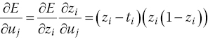
where K is the total number of outputs, t i is the ith target output, and z i is the ith output obtained from the final output layer. The aim now is to find the output that minimises E. The method used is the gradient‐descent with momentum method (Spentzos 2005), which works as follows.
The error change due to a change in the output is found by differentiating Eq. (10.20) and is given by

Therefore, the change in the error due to the change in the input to the node that created z i is
where ![]() is found by differentiating Eq. (10.19), and where z
i
is the equivalent of y
j
for the output layer. Similarly, the change in E due to a change in the hidden‐layer node input (which is similar to x in Eq. (10.19) is
is found by differentiating Eq. (10.19), and where z
i
is the equivalent of y
j
for the output layer. Similarly, the change in E due to a change in the hidden‐layer node input (which is similar to x in Eq. (10.19) is

This is repeated all the way to the first input and the total error is calculated. Then the weights are changed by a small amount, in proportion to the error calculated and the input to each neuron. So w ij can be updated as:
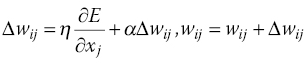
In Eq. (10.24), α is termed the ‘learning momentum’, because it scales up the change in the weight at each iteration (it is multiplied by the previous weight change), and η is termed the ‘learning rate’, because it scales up the movement along the gradient. The higher these values are, the lower the training time required. However, values that are too high can cause instability and a failure to converge. To further improve the speed of training the ANN, it is allowed to skip a number of steps periodically before the weights are modified as a ratio of the last written weights. A further improvement is the use of an adaptive learning rate. This means that the learning rate changes according to the change or gradient in error for each epoch or set of epochs, which allows the training to occur faster when the ANN is learning quickly and slower if it is learning slowly. The learning rate, η, is multiplied by a fraction less than one if the ratio of the present error to the previous error falls above a certain value and greater than one if it falls below a certain value. In this way, η is constantly adapting to the ANN’s learning ability.
Another important parameter to consider in training the ANN is the error convergence. This value must not be smaller than the error resolution of the data points used for training. For example, if the CFD data is accurate to within 1% of its value, then the ANN training must not force the difference between the predicted and target value to be less than 0.01. If so, the ANN prediction trends bend and flex to try and pass through each point inside that tolerance, resulting in over‐fitting and large training times. Figure 10.4 shows a comparison of ANN predictions when trained to different convergence values for a test case, which is described in full in Johnson and Barakos (2011). For the purpose of demonstrating the effects of the ANN parameters, this test case is explained briefly here. The aim was to optimise the camber and thickness values of section of a NACA 5‐digit rotor for a blade in forward flight and using the moment, lift and drag parameters. These loads are compared against the camber parameter. As can be seen in the figure, the best compromise is a convergence value of about 1% in that the trend is captured. A smaller convergence value overfits the data, because it falls within the error tolerance of the training data itself. The length of time for training required increased exponentially with smaller convergence values. The smallest convergence took about 25 times longer than the intermediate, which took approximately six times longer than the biggest convergence value. Also, using a fixed η took the ANN about 1.25 times longer to train. Using the adaptive η results in a different weights file, but the differences in the overall predictions are negligible, as shown in Figure 10.4.
Figure 10.4 Error convergence comparison for an example ANN. This is for the optimisation of a NACA 5‐digit rotor section on a blade in forward flight. The x‐axis is the camber value of the section and the y‐axis is the peak‐to‐peak moment of the section over a full revolution. The various curves and the legend correspond to the training of the ANN to converge at different error values, as well as a comparison with the ANN that had an adaptive learning rate. The black dots represent the data used for training and the pink dots are the accurate CFD data not used in the training set; that is, validation data. The full test case analysis can be found in Johnson and Barakos (2011).
The number of hidden layers and neurons required to get accurate predictions is determined by the physics of the test case, and the number of inputs and outputs (Spentzos 2005). It was found that if more inputs and output variables are used, then a ‘smarter’ ANN is required: one that allows more degrees of freedom. Therefore an increased number of layers and neurons are required. Having too many layers for a small number of inputs and outputs can cause overfitting of the data. Figure 10.5 shows the predictions with different numbers of layers and neurons for a number of outputs belonging to the rotor section test case. The C l and C d curves show that when the output variables are increased, an increase in the number of layers or neurons has approximately the same accuracy as a single‐output prediction with fewer layers or neurons. The green curve is the most inaccurate because it has a large number of outputs and the least number of neurons and hidden layers. Increasing the number of neurons increases the accuracy of the predictions. This is seen more clearly in Figure 10.5c for the average C m . For a single output, the ANN with 2 layers and 21 neurons has a more accurate curve fit than the ANN with 2 layers and 15 neurons. For the 7 output case for the same output in Figure 10.5d, a higher degree of freedom is required and hence an increase in the number of layers is required to get a smooth curve fit through the data, similar to the single‐output prediction. Increasing the number of neurons does not improve the prediction accuracy.


Figure 10.5 Comparison of ANN prediction for scaled average C l , C d and C m with different numbers of outputs (out), hidden layers (hl) and neurons (n). The number of inputs is constant at two. This is for the optimisation of a NACA 5‐digit rotor section on a blade in forward flight. The x‐axis is the camber value of the section and the y‐axis is the average moment, lift and drag of the section over a full revolution. The various curves and the legend correspond to the training of the ANN with different numbers of neurons and layers. The black dots represent the data used for training and the cyan dots are the accurate CFD data not used in the training set: the validation data. The full test case analysis can be found in Johnson and Barakos (2011).
This shows the importance in validating the metamodel before using it in the optimiser. In this work, the metamodel is always validated with additional high‐fidelity data unknown to the metamodel. Once the ANN has been trained, it can then be used to accurately predict the output for any input within the limits used for training.
For large values along the x‐axis of the activation function – in other words, for large input values – the resolution of the output is reduced, as suggested by Eq. (10.17). Hence, for more accurate results, the inputs are normalised to between 0 and 1. Input data that is not within the range of the original data can be predicted as well (extrapolated from the data). These inputs must be included in the data before being normalised, so that all data is always between 0 and 1. These inputs for which the outputs are unknown can be deleted from the data file in the training stage and re‐introduced in the prediction stage. However, it has been found that the ANN is highly inaccurate in predicting extrapolated data, so it is suggested that the outputs of the input parameters on the boundaries of the design space should always be known values.
Once the inputs have been normalised, the normalised data are used to train the ANN. Training can continue until a set epoch number is reached or until the values converge to a pre‐defined error value between the predicted and target results. In this case, training is always carried out until convergence to a specified error margin.
After training the ANN, the final weights are written to a file. This file is used to predict the output for a normalised set of inputs and then the predictions are denormalised to obtain the predicted results.
Polynomial Fit
Given a number of points, the aim is to fit a polynomial curve through them or create a polynomial equation that satisfies all the points given. Hence, the more known points there are, the more reliable the predictions are and the greater the degree of the polynomial can be. For example, if there are only two points, only a straight line can be used to predict data that falls anywhere on the plane. If three points are known, then a quadratic curve can be fitted through the points and hence the predictions are more accurate, and so on. The maximum degree of the polynomial is dependent on the number of points available, the limit being a function of the number of unknowns in a set of simultaneous equations. If (x 1,y 1) (x 2,y 2) and (x 3,y 3) are three points on a plane and a quadratic polynomial is to be fitted through these points, then,
Using Gaussian elimination or lower–upper (LU) decomposition or any other method for solving simultaneous equations, the coefficients A, B and C can be found.
It is possible to use a polynomial to fit non‐linear data. However, if the data do not follow a polynomial trend, having too high a degree of polynomial can result in overfitting the curve. Therefore, normally, the degree of polynomial is limited to six or less (Mathews and Fink 2004).
Figure 10.6 shows a comparison of polynomial fits to the data used to analyse the ANN in Section 10.4.1. With a polynomial of order four, the data are not as accurate as the ANN, but with an order of ten, the polynomial fits closer, although it is less smooth and still not quite as accurate. The advantage of the polynomial technique is that it does not require training time as the ANN does. However, as it is not likely that more than four or five known points will exist for a variable, the order of the polynomial is limited. The ANN will therefore be a better selection for the BERP‐tip example described later in this chapter. The method can be very effective if a law exists for the variation of the output. For example if C d versus C l follows a parabola, then a polynomial can be used.

Figure 10.6 Comparison of ANN prediction accuracy with polynomial of order 4 and 10 for ΔC m . Three hidden layers (hl) and 15 neurons (n) were used for the ANN. Number of inputs is kept constant at two. The solver training and prediction comparison is included.
From Johnson and Barakos 2011.
Kriging
The kriging approximation method is a more complex version of the polynomial fit method. It uses sample data points to build a model that can be used to predict the output or performance of interpolated design points by fitting a low‐order polynomial through the data points but allowing the predictions along these polynomials to deviate based on a correlation model, such as a Gaussian distribution of all the existing points. The Gaussian distribution’s characteristics are based on the correlation between the sample points; in other words, on their proximity to each other. This allows the kriging parameters to change with the prediction point, giving the approach more flexibility while still maintaining accuracy (Lophaven et al. 2002). Assume the output or performance, P, is represented as:
where f(x, y) is the polynomial and Z(x, y) is the correlation model; the latter is based on the Gaussian distribution for all the cases in this chapter. The correlation between all the sample points with each other, and the correlation between the required point and all the points is found as the Gaussian distribution of the distances between all these points with a ‘roughness’ parameter θ for each design parameter. So, Z is actually a function of θ as well as x and y; that is, Z(θ, x, y). All the parameters and values are normalised and then denormalised, at the end, so that the mean of Z(x, y) is 0. Also, the data are normalised in a scalar way over each parameter between 0 and 1. So the correlation between P and F can be described as:
where β can be approximated as:
and the variance can be estimated as:
where m is the number of initial data points. The matrix Z, and β and σ 2 depend on θ, where θ is effectively a width parameter that determines how far the influence of a data point extends (Forrester and Keane 2009). It is similar to a weight put on each input depending on its influence on the output. A low value means there is a high correlation and the influence of each point affects many other points. A large value means there is less correlation and hence it has less influence on another point. In this way, θ can also be used to find the design parameters that have the most influence on the performance parameters.
The optimum value of θ is defined as the maximum likelihood estimator, the maximiser of
where |Z| is the determinant of Z (Lophaven et al. 2002). This value is found iteratively, although for small cases with few inputs, a good estimate can be made by comparing predictions with the original data.
The Gaussian correlation function, Z(x, y) can be found as the covariance matrix:
where i and j are the sample points and r represents the required points, x and y are the design parameters and d is the distance between the points, which in this case is squared; the value to which it is raised can be between 0 and 2 and represents the differentiability of the response function with respect to the design parameters. Values close to 0 indicate that the function is not differentiable or smooth and a value closer to 2 is for differentiable functions (Lophaven et al. 2002).
The weight matrix, λ, which contains all the weights to obtain the required point from each point in the design space, can then be found as
Then, the prediction can be made as the summation of each appropriately weighted objective function value

More details can be found Mantovan and Secchi (2010) and Lophaven et al. (2002). For the polynomial fits, up to order‐two polynomials are common. In some cases, constant values are sufficient, such as the mean value of all the data.
Figure 10.7 compares the data in Figure 10.6 as predicted by the polynomial, ANN and kriging metamodels. The kriging method tends to smooth out the surface more than the ANN, although this can be dealt with by optimising its parameters. Nevertheless, the ANN and the kriging both seem to perform consistently well across all the cases with little change in parameters, slightly more so for the ANN than the kriging method. The advantage of the kriging is that training time is not required. Both methods are capable of making reasonably accurate predictions.
Figure 10.7 Comparison of ANN prediction accuracy with polynomial of order 10 and kriging for ΔC m . Three hidden layers (hl) and fifteen neurons (n) were used for the ANN. Number of inputs was kept constant at two. The solver training and prediction comparison is included. On the right, the blue surface is the ANN prediction and the red is the kriging prediction.
Proper Orthogonal Decomposition
Proper orthogonal decomposition (POD) is a mathematical technique that is used in many applications, including data compression (Lawson 2007). An analogy can be made with the Taylor series or the Fourier transform, where the part of the infinite equation that does not add significantly to the data is neglected. In the case of fluid dynamics, the flow is decomposed into modes. The modes that make major changes to the flow are retained, and the rest are ignored.
The principle behind POD is that any function can be written as a linear combination of a finite set of functions, called basic functions. There are a number of different ways of performing this decomposition, two of which are the Karhunen–Loève decomposition (KLD) and singular value decomposition (SVD) methods. The SVD method can be described as follows.
Let A be the data matrix, an ![]() matrix where
matrix where ![]() . The SVD equation is:
. The SVD equation is:
where U (whose columns are called left singular vectors – output basis vectors for A) is an ![]() matrix, where mo is the number of modes, S (whose diagonal elements are called singular values ordered in decreasing value order) is a
matrix, where mo is the number of modes, S (whose diagonal elements are called singular values ordered in decreasing value order) is a ![]() matrix and V
T
(whose rows are called the right singular vectors – input basis vectors for A) is
matrix and V
T
(whose rows are called the right singular vectors – input basis vectors for A) is ![]() matrix. More details can be found in Lawson (2007).
matrix. More details can be found in Lawson (2007).
The Karhunen–Loève expansion is usually used to represent stochastic processes (in other words, a family of random variables with respect to time) as a combination of random deterministic time functions. The method of snapshots for the KLD method was introduced by Sirovich (Everson and Sirovich 1995). A snapshot is a set of data at certain spatial points at one particular time. So, the data matrix consists of two dimensions, the first being the spatial grid point data and the second being time. The snapshots are taken at regular intervals over the period of flow. In the KLD method, any snapshot can be expanded using eigen functions. Taking velocity as an example,

where u m (x) is the mean velocity, Φ i (x) is the spatial KLD mode and a i (t) is the temporal KLD eigen function. To generate this decomposition, the first step is to calculate the covariance of the input data matrix,
The resulting matrix is symmetric and has dimensions of ![]() . The eigenvalues and eigen vectors of the covariance matrix are then computed. The matrix containing the eigenvectors are temporal KLD eigen functions a
i
(t). The original data matrix is then multiplied by the eigenvector to produce Φ
i
(x). The eigenvalues represent the amount of energy stored in the mode; in other words, its contribution to the overall flow.
. The eigenvalues and eigen vectors of the covariance matrix are then computed. The matrix containing the eigenvectors are temporal KLD eigen functions a
i
(t). The original data matrix is then multiplied by the eigenvector to produce Φ
i
(x). The eigenvalues represent the amount of energy stored in the mode; in other words, its contribution to the overall flow.
Typically enough modes are stored to capture 99% of the energy:

where λ n is the nth eigen value. Generally, the KLD mode is faster and requires fewer modes to reconstruct the flow. Also, it is less sensitive to load imbalance and hence larger block sizes can be used. Even with increased number of snapshots – larger matrices – the KLD execution time increases slower than the SVD method. The number of snapshots has a larger effect on execution time than the number of spatial point data. In addition, a method has been found for compressing data as it is obtained for each time step from the solver, using the SVD method. No such method has been found for the KLD (Lawson 2007).
The POD is not only used as a compression tool to reduce the size of data stored, but can also be used to predict missing data for required inputs, for what has come to be commonly known as ‘gappy’ data (Willcox 2006). From the theory shown, the model is reconstructed using the eigen functions that carry the highest energy. In this case, the aim is to be able to predict the loads of aerofoils that were not solved for using CFD. There are two methods of doing this: the POD/Galerkin method and the POD/interpolation method. The POD/interpolation method is more suitable with data that does not have much correlation (Joyner 2001).
The field data is reproduced as follows:

where U is the data that exists, p is the number of modes used for reconstruction, α i is the ith temporal POD coefficient and Φ i is the ith spatial POD basis vector.
The file containing the original data set (gappy file), U, and the required file are usually organised as the value at each spatial point down; in other words, each row represents the value of U at a different point in space, and for each snapshot or time step across; in other words, each column represents a time step, so that you have a matrix of ![]() . Using, for example, the ΔC
l
values for the aerofoils, the thickness values could replace the spatial data points and the camber values as the snapshots. So, for example, the case described in Section 10.3.4 is used where ΔC
l
is the data matrix for A and it would look like this:
. Using, for example, the ΔC
l
values for the aerofoils, the thickness values could replace the spatial data points and the camber values as the snapshots. So, for example, the case described in Section 10.3.4 is used where ΔC
l
is the data matrix for A and it would look like this:

A mask vector, n k describing where the data is missing must first be created as follows:
where ![]() is the i
th
element of the vector U
k
. Let g be the solution vector that has some elements missing. Then,
is the i
th
element of the vector U
k
. Let g be the solution vector that has some elements missing. Then,

where ![]() is the repaired vector. The error between the data that exists in both the solution with the missing data and the repaired vector is given by E,
is the repaired vector. The error between the data that exists in both the solution with the missing data and the repaired vector is given by E,
Only the existing data are compared, using the mask vector to mask out the new inputs. The coefficient b i is varied so as to reduce the error. b can be found by differentiating Eq. (10.46) with respect to b such that
where ![]() and
and ![]() . Solving this for b gives g and the missing data can be inserted into the original data matrix (Bui‐Thanh et al. 2004).
. Solving this for b gives g and the missing data can be inserted into the original data matrix (Bui‐Thanh et al. 2004).
Now, if a number of snapshots are missing the first step is to fill in the missing data with random values or averaged values for the required points. This data matrix is used to obtain the POD basic vectors. As described above, these matrices are used to obtain a corrected data matrix from Eq. (10.45). The values from these intermediate repaired data are now used to reconstruct the missing data for the next iteration. This is continued until the algorithm converges or the maximum number of iterations is reached. For a more in‐depth explanation of the KLD method, see the work done by Ly and Tran (1998).
This method, however, is reliant on the availability of data in as many positions as possible and requires at least two elements of data in each snapshot. It also does not perform well with few data points. With smaller files, within each snapshot, if in addition to the required point another point is missing, the accuracy of the prediction is highly compromised. For example, take the load, average C m at a thickness of 12% and camber of 23 for the rotor optimisation case described in Section 10.3.4. In the data shown in Table 10.1, the difference is more than double the actual value. This large effect is because the initial matrix is small and so every point missing represents a large portion of the initial matrix.
Table 10.1 Comparison between CFD and ANN predictions for the average pitching moment coefficient.
| Prediction method | Avg C m |
| CFD | 1.296992 |
| 1 point missing | 1.28567 |
| 2 points missing | 3.47769 |
For the matrix shown earlier, predictions were made for the aerofoil of camber 33, thickness 12 and 18 using an ANN and the gappy POD method and compared. The results are shown in Figure 10.8 and, as can be seen, the POD does not perform well with sparse data. Even with a greater number of points, such as 20 variables for each design parameter, which is far above what is practically viable with high‐fidelity CFD software, the ANN has superior performance, as demonstrated here. The ANN predictions of 21 points of average C m were used to show the POD’s dependency on the amount of data available to it, as shown in Figure 10.9. With one point missing, the error is small, but as the number of missing points increases, the error grows. Also, the position of the missing data plays a role. If there are many points missing in one location, as opposed to points spread over the full domain, the error can be larger, as shown in Figure 10.9. This is one of the main advantages that the ANN has over the POD interpolation method, in that even though ANNs require more time for training, the POD would require more points for higher accuracy, which reduces its efficiency.

Figure 10.8 Comparison of ANN and POD predictions trained with the original database of 20 CFD points, less the two that are predicted.

Figure 10.9 Comparison of original data (ANN predictions of average C m for varying NACA aerofoil thicknesses at R = 50%) with POD interpolation predictions, comparing number and position of training data points.
The gappy POD method was originally used to reconstruct images that were ‘damaged’ or unclear, such as face recognition, satellite maps and CFD flow field data. In these cases, more data is available and at a comparatively smaller resolution. Therefore, the POD interpolation technique works well. However, in the case where very little data is available (which is expected when high‐fidelity CFD data is required) the trends are not predicted as accurately as when other methods are used.
10.3.5 Genetic Algorithm Optimisation Method
For the optimisation, a non‐gradient method in the form of a genetic algorithm (GA) was implemented and combined with the metamodels. Figure 10.10 shows the analogy and terminology used as applied to the optimisation of an aerofoil case: selection, crossover, mutation, competition, survival. Two parents are first selected based on a roulette‐wheel technique. The roulette wheel is a file containing the full population of design points. However, each design point takes up as much space (in other words, it is repeated) in the file as is proportional to its fitness or performance by duplication; in other words, the wheel is biased towards fitter individuals. A random selection is made from it, but since the wheel is biased, the evolution leads to better designs being created. The proportionality function for space on the roulette wheel is user‐defined from linear to exponential and is necessary for convergence and stability. This is because if the number of individuals in the database is very high, the percentage of space taken up by fitter individuals on the roulette wheel reduces and the selections become less biased and more random. Therefore a better fitness assignment rule would be an exponential one rather than a linear one, for example.
Figure 10.10 Outline of the genetic algorithm employed for an aerofoil selection case and the analogy with genetics. OFV, objective function value.
Once the parents have been selected, their ‘genes’ are swapped or crossed over. A number of crossover methods have been developed. The most commonly used is random crossover and it is used in this chapter. Here, a gene or more are randomly selected and swapped, producing two new offspring. In the illustration in Figure 10.10, either the thickness or camber is selected randomly and swapped between the two aerofoils.
For the mutation stage, the offspring parameters are converted to binaries of 10 bits, analogous to genes. This representation is simple and effective. In the natural world, the genome is the most basic form of discretisation. Similarly, in the computing world, binary is the basic form of discretisation. A random bit is then chosen and changed to either 1 or 0. Mutation is necessary since it has been found that after a number of generations, some characteristics of the genes get ‘lost’ (Hirsh 1998). Mutation allows for these characteristics to be re‐introduced into the gene pool and it also increases diversity, which allows the global optimum to be found. Its probability is kept low by allowing only one point to be changed and there is a 50% chance that it will be changed to a different value. So the probability of 1 bit changing is 1 in 20 for 10 bits. This prevents the change in the phenotype from happening too often, which would cause the process to lose its evolutionary driving force. The probability of mutation can be increased by selecting more than one point for mutation or by switching the bit in the gene rather than assigning it a value it may already have or by swapping two bits in the code.
The resulting offspring is then assessed by employing the trained ANNs (along with its normalisation and denormalisation functions) and combining their output using the user‐defined objective function. This objective function is then modified to stay within the user‐defined constraints. There are two types of constraint exercised. One type limits the boundaries of the design space so that the predictions of the metamodel are accurate. The other includes physical constraints:
- geometric, such as. thickness, minimum tip chord length
- aerodynamic, such as angle of attack, stall margin, drag‐divergence Mach number.
There are two ways to deal with these constraints: either as hard constraints or as soft constraints (Hajela 1999). Soft constraints are beneficial initially as they increase the diversity of the population, preventing the GA from terminating prematurely before the global optimum is found.
After a number of such iterations, a pool of the offspring characteristics is created and a threshold value is set so that only the majority of the fitter individuals survive and pass on into the next generation pool. The fittest individuals are always carried through into the next generation. This is termed ‘elitism’. While the GA can converge without the help of elitism, the convergence takes longer and has a lower probability of being the global maximum since only mutation is capable of re‐introducing new design characteristics or ‘alleles’ back into the pool, and these may not be the best designs. Using elitism ensures that the best genes still exist in the gene pool (or ‘live longer’) and hence there is a higher probability of reaching the maximum value (Hirsh 1998). Cloning is avoided as it can change the selection process unfairly.
10.3.6 Pareto Front Optimisation
The optimiser used here employs an objective function to determine the optimum and so the selection pressure is towards a small area in the design space. However, another way of finding the optimum is to find the designs that provide the best compromise between all the performance parameters. This is known as the ‘Pareto front’. The advantage of using a Pareto‐front‐type optimiser (PFO) is that it provides a range of design points that represent the best combination of performance measure parameters. In essence, the PFO method provides the user with the designs that give the best performance for each parameter and subsequently leaves the weighting of these performance parameters to be decided at the end of the optimisation process.
The advantage of using an objective‐function‐type optimiser (OFO) is that it allows designs that do not necessarily fall on the Pareto front to be included in the genetic algorithm’s selection, based on the end‐point required. So, rather than spreading out the performance along a front, it clusters it at a specific objective.
For example, in Figure 10.11, if C M has less value in the objective of the design, point 2 is still a good design even though it may not fall on the Pareto front. However, having the Pareto front is a good indicator that there may be a slightly better design, possibly at point 4.
Figure 10.11 Pareto front and objective function optimisers.
10.4 Parameterisation Technique
Parameterisation plays a key part in increasing the efficiency of the optimisation process. The fewer the design variables used to define a shape (for a fixed amount of flexibility), the smaller the initial population of high‐fidelity data (since the number of dimensions of the database is reduced), the less training time required for the metamodels, the more accurate their predictions are given a fixed number of samples, and the faster the output of the optimiser.
Some techniques use fewer parameters. These techniques, however, can reduce the intuitiveness of the shape representation or reduce the flexibility of the design change. For example, splines and NURBS can be used to represent the data quite efficiently for the amount of flexibility available, but the movement of control points and weights is not directly intuitive to how the shape is being changed. However, these methods are very useful for the design of compressor blades, for example, as these are typically defined as splines. Also, high flexibility may not be required if the aim is to fine‐tune specific design parameters rather than to change a shape completely.
Another method uses equations, where the coefficients involved are varied to change the design and the equations are then matched at their end points. This technique allows a lot of flexibility, since any number of equations can be used to define a shape. The matching can be used to reduce the number of independent variables. With experience, these variables can become somewhat intuitive to the change in the shape. This is useful in planform design and was also used by us for the BERP‐like tip and fuselage parameterisation.
Overall, the parameterisation method should be tailored to what best works for each case. Kulfan and Busoletti (2006) discuss a number of methods used to parameterise aerofoils and also discuss a new method of parameterisation. They also listed a number of desirable features of an ideal parameterisation method, referring specifically for aerofoils, (Kulfan and Busoletti 2006), although the characteristics could also be applied to other cases too. These characteristics are shown in Table 10.2.
Table 10.2 Desirable features of an ideal parameterisation method.
| 1. | Well behaved: should produce smooth and realistic shapes. |
| 2. | Mathematically efficient and a numerically stable process that is fast, accurate and consistent. |
| 3. | Require relatively few variables to represent a large enough design space to contain optimum aerodynamic shapes for a variety of design conditions and constraints. |
| 4. | Allows specification of key design parameters such as leading‐edge radius, boat‐tail angle, aerofoil closure (examples specific to aerofoils). |
| 5. | Provide easy control for designing and editing the shape of a curve. |
| 6. | Intuitive – geometry algorithm should have an intuitive and geometric interpretation. |
| 7. | Systematic and consistent – the way of representing, creating and editing different types of geometries must be the same. |
| 8. | Robust – the represented curve will not change its geometry under geometric transformations, such as translation, rotation and affine transformations. |
For the BERP‐like blade equations, each design variable required was independently defined but allowed a smooth curve to be created. The process was automated as described below. Figure 10.1 shows some defining features for the parameterisation of the BERP‐like blade. The parameterisation technique developed for this optimisation process allows for the following design features to vary:
- the sweep angle
- the gradient of the BERP notch
- the spanwise position of the notch.
To do this, both the leading and trailing edges of the BERP tip are modified. Referring to Figure 10.12, the leading edge is defined by three equations and the trailing edge by two. For the leading edge, the first part is defined by a sigmoid curve that represents the notch region. The sigmoid equation is given by:

where
- Δy is the notch height – the notch length in the chord‐wise direction
- Δx is the total width of the notch – the notch length in the spanwise direction
- g is the gradient of the notch
- x o is where the notch starts from.
The x coordinate of the notch maximum is defined by the user and is kept constant except when the notch position needs to be varied. The g value changes the gradient.
Figure 10.12 Definition of BERP‐like design parameters.
The second part is used to define the sweep. It represents the part of the leading edge after the notch as a parabola:
where a is the gradient of the parabola used to alter the sweep, x 1 corresponds to the notch end and the beginning of sweep, Δy is the notch height and y add is an additional y offset value to ensure that the y ordinate of the parabola starts at the same position as the notch height. The value of y add is computed automatically, once x 1 and Δy are known.
The third part describes the delta tip, which joins to the trailing edge. It is represented as a polynomial of order 2.5:
where b is the gradient of the delta tip, c is the centre where the gradient of the curve becomes 0 (used to match the gradient of the curve to the previous parabola) and Δy′ is the additional y displacement required to match the curve to the previous parabolic curve. See Figure 10.12.
The two parameters g and a can be changed independently and the rest of the parameters appearing in the equations are automatically adjusted so that the curves match at the point and have continuity. These are the values of Δx, Δy′ and c. The initial x co‐ordinate, x 0 is modified with the gradient of the parabola so that the tip point occurs at the same place for a required sweep. This is why, for different notch positions, different sweep parameters are used to obtain the same sweep distribution. The gradient b is dependent on the trailing edge curve as well. Therefore, the trailing edge must be determined first. The gradient of the trailing edge curve can also be modified independently of the sweep gradient of the leading edge. This allows the tip point of the blade to move in the y‐direction, which inherently modifies the chord distribution as well.
The trailing edge is defined first by a linear curve that has the same gradient as the leading edge sweep parabola or a scaled value of it, if required, and then by a polynomial of order 3.5 that is matched to the point and gradient of the sweep curve that comes before. The trailing edge curve must be specified before hand, as the tip point is required to find the gradient of the delta polynomial so that the leading and trailing edge curves meet at a single point. So the first curve for the trailing edge is given by:
and the latter part of the trailing edge is given by:
All the values and constants correspond to the trailing edge parameters except for the sweep parameter, a which is exactly the same as the leading edge sweep. The gradient of the trailing edge can be increased or decreased relative to the leading edge sweep gradient by scaling it with a factor. Figure 10.13 shows the examples used to build the design space for the optimisation.
Figure 10.13 Visualisation of the three parameter changes to the geometry surfaces: (a) base rotor with BERP modification; (b) varying the gradient of the notch; (c) varying the sweep; (d) varying the initiation of the notch.
The anhedral and twist of the blade were also modified to match the hover performance of the original blade. Once this was done, these parameters were kept constant; they were not optimised any further. Both values were varied linearly during the grid generation process as described in Section 10.5. Overall, three design parameters were varied for the optimisation. These were the sweep, the notch gradient and the notch position.
10.5 Grid and Geometry Generation
10.5.1 Geometry Generation
Figure 10.13 shows how a swept rotor tip can be transformed into a BERP‐like tip and the effect of varying the parameters. The base rotor is made up of two sections: the HH‐02 inboard (up to r/R = 0.92) and the NACA 64A‐006 at the tip (r/R = 1). The aerofoil is linearly blended towards this latter section. This rotor has a rectangular tip, swept back by 20°, as shown in Figure 10.14. When the BERP planform is applied to this tip, the non‐linear variation of the chord means that the thickness changes non‐linearly as well. To maintain the thickness so that it decreases linearly, from 9.6% (thickness of the HH‐02) to 6% (thickness of the NACA 64A‐006), sections are cut from the base rotor such that when they are scaled to the chord length required, they have the thickness value that satisfies the linear variation. The problem with this method is that the point of maximum thickness for each of these sections varies non‐linearly, and therefore the blade surface appears to be bumpy. To overcome this, the notch section is blended from the HH‐02 to a NACA‐64A section of the appropriate thickness and then the rest of the tip is built with NACA‐64A sections of the required thickness so that, at the tip, the thickness is 6%.
Figure 10.14 Schematic of the baseline rotor blade.
Another issue that arises is that the HH‐02 aerofoil has a tab whilst the NACA 64A‐006 does not. So a tab is introduced for the NACA64A and is kept constant until where the tip is rounded off. The tab is introduced by cutting the aerofoil curves at about 20% from the trailing edge and then rotating the latter part of the curves in the longitudinal axis of the blade so that it adds the required thickness for the tab. The curve is then blended by point, tangent and radius to the main part of the curve to remove any kinks.
ICEMCFD™, a geometry and blocking generation software, was used to build the grid. ICEMCFD™ allows automation via ‘replay files’. A number of the steps in the grid building exercise were automated in this way, although some manual intervention was required to finalise the grids.
10.5.2 Tip Anhedral
The tip anhedral is implemented as follows. Assuming that 40![]() of anhedral is to be implemented starting from the station r/R = 0.918 to the tip. For each station in between these two stations (r/R = 0.918 and r/R = 1.0), there will be a Δz distance by which that section should be translated downwards (Figure 10.15) which is found as:
of anhedral is to be implemented starting from the station r/R = 0.918 to the tip. For each station in between these two stations (r/R = 0.918 and r/R = 1.0), there will be a Δz distance by which that section should be translated downwards (Figure 10.15) which is found as:
Once each station has been translated, then the stations are joined by curves and surfaces are created.
Figure 10.15 Generation of anhedral for the blade tip.
10.5.3 Mesh Generation
The blocking used is of the multiblock type, whichconsists of a C‐type topology around the blade set inside an H‐type topology containing the full flow domain. Figure 10.16 shows the blocking for a single blade. This was copied and rotated around the azimuth to form a rotor of four blades, which were then used in the computation. Details of the mesh size in the farfield and on the blade are also shown. The total grid size was approximately 11 million cells for all four blades. The spacing perpendicular to solid surfaces was ![]() of a chord length, resulting in
of a chord length, resulting in ![]() . The Reynolds number variation is expected to be between 5 and 10 million for forward flight. Figure 10.16 shows the rounded tip and trailing‐edge tab for the blade.
. The Reynolds number variation is expected to be between 5 and 10 million for forward flight. Figure 10.16 shows the rounded tip and trailing‐edge tab for the blade.

Figure 10.16 BERP‐like blade: (a) block boundaries; (b) mesh details.
10.6 Flight Conditions
The hover flight conditions for the blade were based on a rotor‐tip Mach number of 0.65, which was assumed from a tip speed of 220 m/s at International Standard Atmosphere (ISA) sea‐level conditions. The chord of the blade root was 0.534 m and therefore the corresponding Reynolds number was approximately 8 million. The weight of the aircraft was estimated to be 9000 kg; that is, the maximum weight in hover. This results in a C T of 0.018 based on a rotor radius of 7.32 m.

For forward flight, an advance ratio of ![]() is selected. This represents a relatively high‐speed case, where the performance of swept and BERP blades is of interest. The thrust value for forward flight was based on approximately half the maximum hover weight.
is selected. This represents a relatively high‐speed case, where the performance of swept and BERP blades is of interest. The thrust value for forward flight was based on approximately half the maximum hover weight.
These conditions are rough estimates and not exact values for a forward‐flying aircraft, because the optimisation process is not being applied for a specific aircraft case.
10.7 Hover Results
First, the hover performance of the original blade was analysed and compared to that of the reference BERP‐like blade. For the hovering rotor, the wake is assumed to be steady and the calculations were performed in steady‐state mode. Also, it is assumed that the flow is spatially periodic and therefore a 1/N
blade segment of the full flow field is used with periodic boundary conditions. The boundary conditions for the farfield boundaries employ a source–sink model (Steijl et al. 2006). These conditions were prescribed at a distance of four rotor radii away from the rotor plane and for the outflow, a potential sink or ‘Froude’ condition was used (Srinivasan 1994). A quarter segment of the rotor and its surrounding field was created, similar to that shown in Figure 10.16. The mesh size was approximately 9 million cells with 300 cells surrounding the sections on the blade, with a perpendicular spacing of ![]() chords.
chords.
The objective was to match or better the hover performance in terms of FM over a range of thrust settings using twist and anhedral and not the design parameters to be optimised for in forward flight. This new twist and anhedral blade will then be used to optimise the planform for forward flight. The FM over a range of thrusts was obtained for the original rotor and a BERP variant. Figure 10.17 shows the comparison of the CFD results of these blades for increasing C T /σ, where σ is the rotor solidity. No experimental data was available for validation. Therefore the results only serve as a relative comparison. The BERP rotor with the same twist and anhedral has a better FM at low thrust. However, at higher thrust values, its performance drops to below that of the original rotor. This means that implementing the BERP‐like tip planform reduces the hover performance of the helicopter. However, with a higher twist, the performance of the original rotor is recovered and with an anhedral of 20° implemented, it matches the performance of the original rotor.

Figure 10.17 Figure of merit vs. thrust coefficient of the original and the BERP variants.
The reason for this performance trend is that for the BERP rotor, the loading of the blade increases steeply where the BERP section begins, as can be seen in Figure 10.18. Also the loading inboards is lower than the original rotor. With increasing twist, the inboard loading is increased, which improves the FM. The anhedral reduces the outboard loading and thus the performance of the BERP blade matches the original rotor blade.
Figure 10.18 Lift distribution along the span with varying twist at 13° of collective.
10.8 Forward Flight Results
In this part, the effect of each of the parameters – tip sweep, notch offset and notch gradient – is analysed before the optimisation is presented. The rotor was trimmed manually to give the same C T /σ value by adjustment of the collective angle. This corresponds to the thrust value mentioned in Section 10.6. In all cases, the torque includes pressure and viscous components.
Tip‐sweep Effects
Table 10.3 shows the effect of sweep on the performance parameters of the BERP rotor. There was considerable loss in thrust with increased sweep. Therefore, for all cases, the rotor was trimmed to give the same thrust of approximately ![]() . The obtained loads were very close in terms of C
T
/σ (within 5%). The rolling and pitching moments did not change much and were therefore already well trimmed. The results comparing the effect of sweep are shown in Figure 10.19 for the cases with the highest notch gradient and the most inboard notch positions. With more sweep, it can be seen that the lifting load distribution is reduced at the back and outboards on the advancing side, and increased at the front of the disk and more inboards on the advancing side. The pitching moment is mostly negative on the advancing side and mostly positive on the retreating side. With increased sweep, the moment magnitude increases since moment is calculated about the blade pitch axis.
. The obtained loads were very close in terms of C
T
/σ (within 5%). The rolling and pitching moments did not change much and were therefore already well trimmed. The results comparing the effect of sweep are shown in Figure 10.19 for the cases with the highest notch gradient and the most inboard notch positions. With more sweep, it can be seen that the lifting load distribution is reduced at the back and outboards on the advancing side, and increased at the front of the disk and more inboards on the advancing side. The pitching moment is mostly negative on the advancing side and mostly positive on the retreating side. With increased sweep, the moment magnitude increases since moment is calculated about the blade pitch axis.
Table 10.3 Effect of blade‐tip sweep on performance.
| NE | NG | Sweep | C T /σ | C Q | Avg M 2 C M | ΔM 2 C M |
| 11.75 | 28 | 0.09 | 0.0905 | 0.000192 | 0.002527 | 0.010297 |
| 11.75 | 28 | 0.13 | 0.0900 | 0.000191 | 0.001640 | 0.010290 |
| 11.75 | 28 | 0.21 | 0.0899 | 0.000186 | 0.000197 | 0.011147 |
NE, notch position parameter; NG, notch gradient parameter. Average M 2 C M is over one revolution and ΔM 2 C M is the peak‐to‐peak difference over one revolution.

Figure 10.19 M 2 C n , M 2 C m and M 2 C q for NE = 11.5, NG = 35 and variable sweep. The black line indicates the 0 value.
The torque distribution shows a drop in C Q near the blade notch. C Q is at its highest at the back of the disk before the notch and lowest at the notch near the advancing side. These extremes increase in magnitude with more sweep. Overall, on the advancing side, the torque reduces with increased sweep and on the retreating side reaches maximum value. The moment distribution has similarities to that of the torque and its magnitude is much higher at the front and back for the more swept tips. The lifting load distributions differ much less than the other performance parameters. So one of the tasks of the optimisation algorithm is to find a good compromise between these two extremes. Figure 10.20 compares the blade loads at four azimuth positions to show the effect of sweep at each. High sweep offloads the tip at the back of the disk and increases it at the front. On the advancing side, lift is maintained till just after the notch, where the highly swept blade loses lift quickly. The torque is low for higher sweep at the tip of the blade. The pitching moment has a more positive value at the tip with more sweep and does not have much of an effect inboards.

Figure 10.20 Comparisons of the M 2 C n , M 2 C m and M 2 C q with NE = 11.5, NG = 28 and variable sweep.
Effect of Notch Offset
Note that in Table 10.4, the sweep values differ because the gradient of the parabola differs when the position of notch changes to maintain the same sweep. In the Table, the comparison is shown for the highest sweep value for each rotor with a different notch position. The blade tip for these parameters can be seen in Figure 10.21. Figure 10.22 compare the loads when the notch is more inboards. These are trimmed results although thrust does not change much with notch position as shown in Table 10.4. The effect of the notch offset parameter is to amplify the effect of the sweep parameter. For example, the redistribution of lift is reduced at the back and increased at the front of the disk. This is caused by the sweep being larger in magnitude when the notch begins further inboard. The same can be seen for the blade pitching moment in Figure 10.22 where the region near the edge of the disk, where moment is higher, is thinner for the more outboard notch.
Table 10.4 Notch position effect on performance.
| NE | NG | SWEEP | C Q | Avg M 2 C M | ΔM 2 C M |
| 11.50 | 28 | 0.185 | 0.000186 | 0.000296 | 0.011556 |
| 11.75 | 28 | 0.21 | 0.000186 | 0.000197 | 0.011147 |
| 11.00 | 28 | 0.25 | 0.000184 | 0.000468 | 0.010621 |
NE, notch position parameter; NG, notch gradient parameter. Average M 2 C M is over one revolution and ΔM 2 C M is the peak‐to‐peak difference over one revolution. C T /σ = 0.09.
Figure 10.21 Maximum value sweep comparison for each notch offset value.

Figure 10.22 M 2 C n , M 2 C M and M 2 C Q for NG = 35 and high sweep. The black line indicates the 0 value.
For blade torque, the trend is an increase with more outboard position. Where the notch occurs there is a drop in torque and then a continued increase towards the tip. With a more outboard notch, the torque continues to rise for longer prior to reaching the notch, therefore the latter part of the curve is higher. This can be seen in Figure 10.22 where the value of the increased region just before the notch is higher when the notch is more outboard. Also, the torque further out from the notch is higher for the rotor with the more outboard notch. More inboards, on the advancing side, a decrease in torque is observed over a larger region and this brings the total value of the torque down as shown in Table 10.4.
Table 10.4 also shows that the peak‐to‐peak moment decreases (also seen in Figure 10.20) but the absolute average moment over a full revolution increases, the further outboard the notch is.
Effect of Notch Gradient
Figure 10.23 compares the performance of different notch gradients. The notch gradient has a smaller influence on the design than the other parameters tested. With a higher notch gradient, there is a slight decrease in negative pitching moment, evident from Table 10.5 where the average moment is slightly higher and the peak‐to‐peak value is lower, suggesting that a higher notch gradient provides better performance. The torque is not affected much at low sweep, but at higher sweep, the notch gradient has slightly more influence on the torque, as shown by comparing the top and bottom halves of Table 10.5. This suggests that NG has higher significance for designs with more sweep.

Figure 10.23 M 2 C n , M 2 C M and M 2 C Q for NE = 11.75 and SW = 0.21 with varying NG.
Table 10.5 BERP spanwise notch gradient performance comparison.
| NE | NG | SWEEP | C T /σ | C Q | Avg M 2 C M | ΔM 2 C M |
| 12.00 | 25 | 0.10 | 0.0909 | 0.000189 | 0.002561 | 0.009611 |
| 12.00 | 28 | 0.10 | 0.0907 | 0.000189 | 0.002464 | 0.009566 |
| 12.00 | 35 | 0.10 | 0.0911 | 0.000189 | 0.002357 | 0.009489 |
| 11.75 | 25 | 0.21 | 0.0898 | 0.000188 | 0.000295 | 0.010960 |
| 11.75 | 28 | 0.21 | 0.0898 | 0.000186 | 0.000197 | 0.011147 |
| 11.75 | 35 | 0.21 | 0.0898 | 0.000187 | 0.000105 | 0.011019 |
NE, notch position parameter; NG, notch gradient parameter. Average M 2 C M is over one revolution and ΔM 2 C M is the peak‐to‐peak difference over one revolution. C T /σ = 0.09.
Overall Performance Comparison
Figures 10.24 and 10.25 are a summary of the integrated loads of pitching moment and torque over the blade during one revolution for all three design parameters. The peak‐to‐peak moment value reduces with further outboard notch position and the average moment tends to be more centred around zero when sweep is higher. The torque seems to be mostly affected by sweep on the advancing side. On the retreating side, the differences are more subtle. As a rough initial analysis, this data suggests that a highly swept blade would be optimal. Having a higher notch gradient would also improve the moments and having a notch more inboards would amplify the effects of the sweep. The quantities of the design parameters that make up the optimum design are obtained in the next section.
Figure 10.24 M 2 C M integrated over the full blade at each azimuth.
Figure 10.25 M 2 C Q integrated over the full blade at each azimuth. Both pressure and viscous components are included.
10.9 Planform Optimisation
The original population obtained from the CFD results contained 27 points. The performance components that make up the objective function selected were the average pitching moment (C mavg), peak‐to‐peak pitching moment (ΔC m ) and the torque coefficient (C q ). The objective function weights were determined such that on average each of these components has the same influence. This was determined using the data from the original population that was obtained using the high‐fidelity CFD solver. First each design was scaled with the baseline design case. The baseline case chosen was a BERP that had similar sweep, the most outboard notch position and the least notch gradient in comparison to the original rotor (the rectangular swept blade) shown in Figure 10.26. The parameters were NE = 12, NG = 25, SW = 0.25. The average ratio of C mavg to ΔC m was found to be 2.7893:1 and the average ratio of ΔC m to C q was found to be 0.9548:1. Therefore, the ratio of C mavg to ΔC m to C q is obtained as: 2.6634 : 0.9548 : 1.0000. The weight for C q was then calculated as:
Hence the weights of C mavg and ΔC m are given as:
C q was used as a soft constraint as well. In other words, if it exceeded the reference rotor’s C q , then the objective function value (OFV) was penalised. Since the rotors were trimmed to a C T /σ = 0.09, C T /σ did not need to be constrained. From this data, it was determined that the most influential design parameter was the sweep, followed by the notch position and then the notch gradient. ANNs were trained for each of the performance parameters, as shown in Figure 10.27. The white dots are the GA optimal selection and the black dots are the CFD training data for the ANNs. The dashed line is where the contour level is equal to 1; that is, the value for the baseline design. Each ANN was used to predict a single output with the three available design parameters as inputs. They each consisted of 15 neurons with 2 hidden layers and a convergence tolerance of 1% within the training data. An automatically adjustable learning rate was used to improve the training time required.
Figure 10.26 Baseline BERP‐like rotor compared to a swept‐tip design. (NE = 12, NG = 25, SW = 0.15).

Figure 10.27 ANN predictions with training data and GA selection: (a) C q , (b) scaled average C m , (c) scaled ΔC m .
The performance parameters were used to find the optimum blade using a GA, and the results were compared with the Pareto front shown in Figures 10.28 and 10.29a. It is clear from Figure 10.28 (the white dots are the GA optimal selection and the black dots are the Pareto front solutions) that selecting an optimum design from the Pareto front when there are several design parameters can still be a difficult task. On the other hand, a weighted function makes it easier to find a particular optimum from the designs that also overlap a part of the Pareto front. The overlap is more clearly seen in Figure 10.29a. The comparison of the optimum with the original baseline blade is shown in Table 10.6 for the trimmed rotors. A much better average M 2 C m was obtained for a slight loss in ΔM 2 C m; at the same time, the torque and thrust coefficient differences are less than 0.5%. The performance of the resulting optimum relative to the baseline design is visualised in Figures 10.29b and 10.30a, which show the difference between the optimum and reference rotor values. The black line indicates the contour line where the difference is 0. Higher values indicate the optimum rotor has a higher value and vice versa. On the moment plot, it can be seen that the optimised blade has higher moments on the advancing side. This is to counter the drop in moments that are experienced on the advancing side (see Figure 10.24). The opposite is true on the retreating side but to a smaller scale since the moments are not as far from zero as on the advancing side. For the torque, the decrease in torque for the optimum blade is almost the same as the areas where there is an increase, leading to very little change in the overall torque.
Figure 10.28 Pareto front points compared with GA selection for (a) NE = 11.5, (b) NE = 11.75, (c) NE = 12.

Figure 10.29 (a) Pareto front for the BERP‐like design. (b) Difference in M 2 C m for the baseline and the optimum rotor.
Table 10.6 BERP and baseline blade (NE = 12, NG = 25, SW = 0.15) performance comparison related to Figure 10.29(b) and 10.30(a).
| NE | NG | SWEEP | C T /σ | C q | avg M2CM | ΔM 2 C m | |
| Optimised | 11.75 | 35 | 0.21 | 0.0832 | 0.000171 | –0.000373 | 0.01078 |
| Optimised | After trimming to 0.09 | 0.0898 | 0.000187 | –0.000105 | 0.01102 | ||
| Baseline | 12.00 | 25 | 0.15 | 0.0905 | 0.000186 | –0.000517 | 0.01083 |
| Hover Performance Comparison | |||||||
| NE | NG | SWEEP | C T /σ | FM | Collective (deg) | ||
| Optimised | 11.75 | 35 | 0.21 | 0.29 | 0.687 | 13 | |
| Baseline | 12.00 | 25 | 0.15 | 0.30 | 0.654 | 13 | |
a NE is the notch position parameter
b NG is the notch gradient parameter
c Average M2CM is over one revolution
d ΔM2CM is the peak‐to‐peak difference over one revolution.
Figure 10.30 (a) Difference in M 2 C q for the baseline and the optimum rotor. (b) Difference in OFV for the baseline and BERP‐like rotor.
Figure 10.30(b) shows the difference in the objective function components between the optimum and the baseline design. From the scale itself, it is observable that there is an overall increase in the OFV due to the optimisation. The figure also shows the regions where there is an increase in the OFV. This is around the notch region, the sweep region and more inboards on the advancing side and front of the disk.
The hover performance of the optimum blade was computed and compared to the baseline in Table 10.6. The results were obtained at a collective of 13°. The C T /σ is slightly less than the baseline design mostly due to the added solidity, but the FM obtained was not substantially changed. Figure 10.31 compares the Cp distribution for the BERP reference and optimised blades at high thrust (the collective was 13°). It can be seen that the optimised planform spreads the loading at the tip over more of the span due to its inboard notch and its higher sweep and reduced tip area. Also from the normal and torque distribution curve, it can be seen that the optimised blade has a reduced load at the tip as well as a reduced torque. Both lead to a very slightly improved Figure of Merit.
Figure 10.31 Reference and optimised blade at high thrust: (a) C P distribution comparison; (b) planform comparison; (c) lift and drag distribution along the span of the blade.
Therefore, overall, the optimised blade has better performance than the baseline blade especially in terms of moment where the average pitching moment was reduced to approximately a fifth of the baseline designs.
The ANN predictions were also very accurate. The error in the ANN convergence during training, was set to 1% for each variable and the maximum error in the overall combined objective function between the CFD data and the ANN predictions was 2.7% which was for a design that had a 16% change in design parameters. This suggests that the ANN is a viable metamodel.
10.10 Summary and Conclusions
This chapter has described the optimisation of a BERP‐like rotor planform using an optimisation method that employed a genetic algorithm and an artificial neural network that was trained using high‐fidelity CFD data from the Helicopter Multiblock Solver CFD solver. The optimisation was carried out for fast forward‐flight conditions. The hover performance was first maintained by modifying twist and anhedral. A parameterisation method was then defined to modify the sweep, the notch gradient and the notch position of the BERP‐like tip. A full factorial method was used to obtain the sample space, which contained 27 design points. The objective was to reduce the compressibility effects on the advancing side of the rotor and stall in the retreating side. This objective was captured using the average pitching moment and the peak‐to‐peak pitching moment of the rotor over a full revolution. In addition, torque was optimised for and constrained. All cases were trimmed to the same rotor thrust. The outcome was a substantially improved pitching moment performance with slightly reduced torque for the same thrust. This was obtained using high sweep and notch gradients with the notch position at approximately r/R = 0.86. Hover performance was not compromised.
The time required to obtain all the data was reduced by using the harmonic balance method and parallel computing. This reduced the the clock time for obtaining the CFD data by an order of magnitude, taking approximately 18 hours when started from a previous solution, compared to 150 hours for time marching over two revolutions (so that the data is periodic). The azimuth resolution for the harmonic balance method was every 10°. This makes the method practical for rotor optimisation in forward flight.
The overall optimisation was limited to the aerodynamic performance of various planform designs and did not include rotor section optimisation. Moderate notch gradient combined with increased sweep resulted in an improvement of the average pitching moment of 80%, although there was an increase of 1.7% in the peak‐to‐peak moment. The torque did not change much and the hover performance was maintained.
These differences in performance can be just as significant, if not more, for UAVs. They can improve the manoeuvrability and control of UAVS, which increases their agility, as well as their efficiency and endurance.
Bibliography
- Brocklehurst A and Duque EPN 1990 Experimental and numerical study of the British Experimental Rotor Programme blade AIAA 8th Applied Aerodynamics Conference, Portland, Oregon, USA. AIAA‐90‐3008.
- Bui‐Thanh T, Damodaran M and Willcox K 2004 Aerodynamic data reconstruction and inverse design using proper orthogonal decomposition. AIAA Journal 42, 8.
- Cameron L, Early JM and McRoberts R 2011 Metamodel assisted multi‐objective global optimisation of natural laminar flow aerofoils 29th AIAA Applied Aerodynamics Conference, Honolulu, Hawaii.
- Caradonna FX and Tung C 1981 Experimental and analytical studies of a model helicopter rotor in hover. Technical report, NASA.
- Daskilewicz MJ and German BJ 2012 Observations on the topology of Pareto frontiers with implications for design decision making 50th AIAA Aerospace Sciences Meeting including the New Horizons Forum and Aerospace Exposition, Nashville, Tennessee, USA. AIAA 2012‐0148.
- Everson R and Sirovich L 1995 The Karhunen‐Loève procedure for gappy data. Journal of the Optical Society of America A 12, 1657–1664.
- Forrester A, Sóbester A and Keane A 2008 Engineering Design via Surrogate Modelling – a Practical Guide. John Wiley.
- Forrester AIJ and Keane AJ 2009 Recent advances in surrogate‐based optimization. Progress in Aerospace Sciences 45, 50–79.
- Hajela P 1999 Nongradient methods in multidisciplinary design optimization – status and potential. Journal of Aircraft 36(1), 255–265.
- Harrison R, Stacey S and Hansford B 2008 BERP IV the design, development and testing of an advanced rotor blade American Helicopter Society 64th Annual Forum, Montreal, Canada.
- Hirsh R 1998 GADO: A Genetic Algorithm for Continuous Design Optimization PhD thesis State University of New Jersey.
- Jang JS, Choi S, Kwon HI, Im DK, Lee DJ and Kwon JH 2012 A preliminary study of open rotor design using a harmonic balance method 50th AIAA Aerospace Sciences Meeting including the New Horizons Forum and Aerospace Exposition, Nashville, Tenessee, USA. AIAA 2012‐1042.
- Johnson C and Barakos G 2011 A framework for optimising aspects of rotor blades. The Aeronautical Journal 115(1165), 147–161.
- Joyner M 2001 An Application of a Reduced Order Computational Methodology for Eddy Current Based Non‐destructive Evaluation Techniques PhD thesis North Carolina State University.
- Kulfan BM and Busoletti JE 2006 Fundamental parametric geometry shape representations for aircraft component shapes 11th AIAA/ISSMO Multidisciplinary Analysis and Optimization Conference, Portsmouth, Virginia. AIAA 2006‐6948.
- Lawson SJ 2007 Parallel performance of library algorithms for computational engineering Master’s thesis University of Edinburgh and Liverpool.
- Lophaven SN, Nielson HB and Søndergaard J 2002 DACE, A MATLAB kriging toolbox, version 2.0. Technical Report IMM‐TR‐2002012, Technical University of Denmark.
- Ly HV and Tran HT 1998 Proper orthogonal decomposition for flow calculations and optimal control in a horizontal CVD reactor. Technical report, CRSC.
- Mantovan P and Secchi P 2010 Complex Data Modeling and Computationally Intensive Statistical Methods. Springer‐Verlag.
- Mathews JH and Fink KD 2004 Numerical Methods Using MATLAB. Pearson Education.
- Mengistu T and Ghaly W 2008 Aerodynamic optimization of turbomachinery blades using evolutionary methods and ANN‐based surrogate models. Journal of Optimization Engineering 9, 239–255.
- Oyama A, Nonomura T and Fujii K 2010 Data mining of Pareto‐optimal transonic airfoil shapes using proper orthogonal decomposition. Journal of Aircraft 47(5), 1756–1762.
- Perry FJ, Wilby PG and Jones AF 1998 The BERP rotor – how does it work, and what has it been doing lately. Vertiflite 44(2), 44–48.
- Régnier J, Sareni B and Roboam X 2005 System optimization by multi‐objective genetic algorithms and analysis of the coupling between variables, constraints and objectives. International Journal for Computation and Mathematics in Electrical and Electronics Engineering 24(3), 805–820.
- Robinson K and Brocklehurst A 2008 BERP IV – aerodynamics, performance and flight envelope 34th European Rotorcraft Forum, Liverpool, UK.
- Samad A and Kim KY 2008 Shape optimization of an axial compressor blade by multiobjective genetic algorithm. Proceedings of the Institution of Mechanical Engineers Part A: Journal of Aerospace Engineering 222, 599–611.
- Samarasinghe S 2006 Neural Networks for Applied Sciences and Engineering – From Fundamentals to Complex Pattern Recognition. Auerbach Publications.
- Simpson TW, Peplinski JD, Koch PN and Allen JK 2001 Metamodels for computer‐based engineering design: Survey and recommendations. Engineering with Computers Journal 17, 129–150.
- Spentzos A 2005 CFD Analysis of 3D Dynamic Stall PhD thesis University of Glasgow.
- Srinivasan GR 1994 A free‐wake Euler and Navier‐Stokes CFD method and its application to helicopter rotors including dynamic stall. Technical Report 93‐01: AD‐A278 000, JAI Associates.
- Steijl R and Barakos G 2008 Sliding mesh algorithm for CFD analysis of helicopter rotor–fuselage aerodynamics. International Journal for Numerical Methods in Fluids 58, 527–549.
- Steijl R, Barakos G and Badcock K 2005 A framework for CFD analysis of helicopter rotors in hover and forward flight 31st European Rotorcraft Forum, vol. 91.
- Steijl R, Barakos G and Badcock K 2006 A framework for CFD analysis of helicopter rotors in hover and forward flight. International Journal for Numerical Methods in Fluids 51, 819–847.
- Tan KC, Lee TH and Khor EF 2002 Evolutionary algorithms for multi‐objective optimization: Performance assessments and comparisons. Journal of Artificial Intelligence 19, 253–290.
- Willcox K 2006 Unsteady flow sensing and estimation via the gappy proper orthogonal decomposition. Computers and Fluids 35, 208–226.
- Woodgate M and Barakos GN 2009 Implicit CFD methods for fast analysis of rotor flows 36th European Rotorcraft Forum, Paris, France.
- Zhao H, Wang S, Han W and Feng G 2008 Aerodynamic design by jointly applying s2 flow surface calculations and modern optimization methods on multistage axial turbines. Frontiers of Energy and Power Engineering in China Journal 2(1), 93–98.