
4
Nonlinear Reduced‐order Aeroservoelastic Analysis of Very Flexible Aircraft
Nikolaos D.Tantaroudas1 and Andrea DaRonch2
1 European Dynamics, SA, Athens, Greece
2 University of Southampton, Southampton, UK
This chapter overviews the technical difficulties that aerospace engineers have to face during the design of environmentally friendly aerial vehicles. Present trends in aerospace design are driven by two factors: increasing the global aerodynamic efficiency and reducing the structural weight to a minimum. The failure in flight of some prototypes of very flexible aircraft, as described in Section 4.1, has shown that traditional (linear) methods are no longer adequate for the analysis and design of future aerial platforms. In Section 4.2, the reader will be introduced step by step to the mathematical models needed to predict the complex interactions that may occur between the aerodynamic, structural, flight mechanical, and control fields. The computational costs of these models, however, are high because of the large number of calculations needed to ensure structural integrity over the flight envelope, and such computational costs are not viable for industrial aircraft design. The latest developments in the field of model reduction will be discussed in Section 4.3, and the reader will have the opportunity to practice and use these mathematical models, utilising the programming codes associated with this chapter. Finally, active control techniques to enhance the performance and resilience of a very flexible aircraft test case to atmospheric gust and turbulence are discussed in Section 4.4. After the conclusions are given in Section 4.5, some exercises are provided in Section 4.6, which can be solved using the programming codes accompanying this chapter.
The chapter is intended to provide the reader with the essential knowledge required to design high‐altitude long‐endurance (HALE) vehicles, which have gained considerable attention in recent years. However, it is worth noting that the mathematical models developed within this chapter are applicable to any aircraft configuration and, in particular, to large transport aircraft with their increasingly larger aeroelastic effects. The generality of the models described here allows more traditional (rigid) aircraft configurations – a subset of very flexible aircraft – to be dealt with too.
4.1 Introduction
The interest in HALE vehicles has increased steadily over recent years because they provide low‐cost efficient platforms for a variety of applications. Their low structural mass and high aerodynamic efficiency allow fight at high altitudes and low speeds with minimal energy consumption. The range of applications of HALE aircraft varies from monitoring and collecting data of the atmospheric environment to rescue missions in biohazard environments. The advantage of unmanned HALE aircraft is the ability to operate at extreme conditions for long duration times without putting at risk human life.
The analysis and design of HALE aircraft, however, presents some unique challenges that are not critical for more rigid (and stiff) aircraft. The dynamic interactions between deformable wings, flow development and flight mechanics may cause structural failure, as occurred in 2003 in the NASA ‘Helios’ prototype. The Helios aircraft was developed under the Environmental Research Aircraft and Sensor Technology (ERAST) program as a HALE‐class vehicle. It was a proof‐of‐concept solar‐electric‐powered flying wing designed to operate at high altitudes for long‐duration flights. Two configurations were produced, the first designed to achieve high‐altitude flight and the second to achieve long‐endurance flight. On 13 August 2001, the first Helios configuration flew at a record altitude of 96,863 ft above sea level. The second configuration was lost in flight on 26 June 2003 after encountering low‐level turbulence. Approximately 30 min into the flight, atmospheric turbulence caused larger than expected wing deformations and the aircraft began a slowly diverging pitch oscillation. The wing dihedral angles remained high and the oscillations never subsided. Instead, they grew with each period and this led the structure of the aircraft and the skin to pull apart, see Figure 4.1.

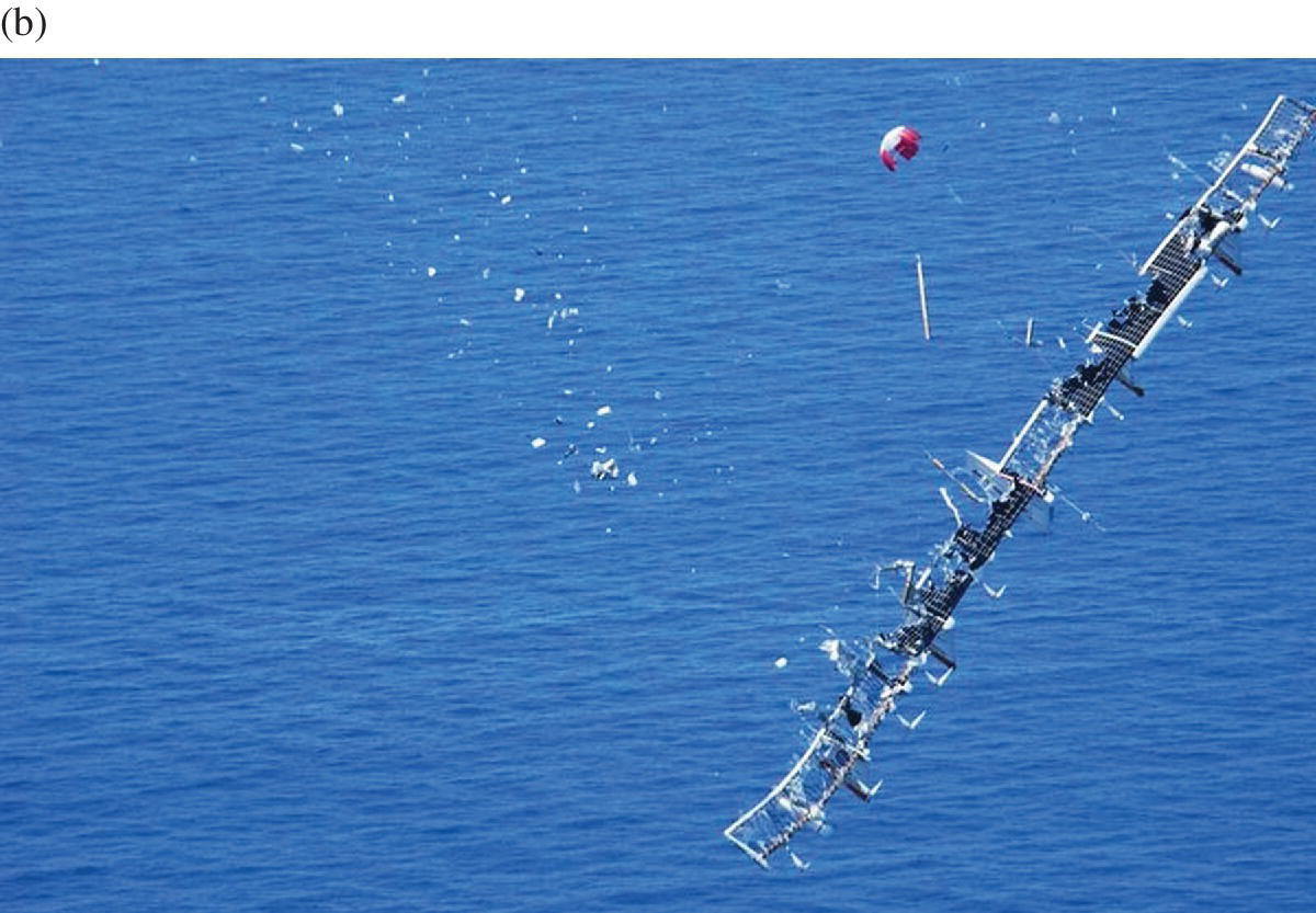
Figure 4.1 The NASA Helios prototype.
From Noll et al. (2004).
4.1.1 Challenges and Prospects
From a technical standpoint, the challenges to be overcome in the analysis and design of HALE aircraft can be summarised as follows:
- The development of a multidisciplinary framework to realistically model the nonlinear interactions occurring between the fluid, structure, flight dynamics, and control fields.
- The lack of an approach to systematically reduce large computational models to a smaller system for faster simulation times and for control synthesis design.
- The exploitation of advanced control design strategies to tame aeroelastic phenomena and improve the effectiveness of the controlled response to atmospheric gusts and extend the flight envelope.
To define the state of the art in the design of HALE vehicles and identify opportunities for progress, a brief review of recent developments in the field is first considered.
Nonlinear Time‐domain Multidisciplinary Framework
There is a large body of work on the development of multidisciplinary frameworks to predict the dynamic response of free‐flying flexible aircraft as they encounter atmospheric gusts and turbulence. Three representative references are those of Dillsaver and Cesnik (2011), Cook et al. (2013) and Tantaroudas et al. (2014). While a nonlinear formulation is generally used for the structural model, which is based on a beam stick representation of the aircraft components, and for the flight dynamics, the aerodynamic model in most studies is inferred from linear assumptions. It is now recognised that the ability to obtain realistic (nonlinear) flow predictions is a key remaining issue in the field of very flexible aircraft. Unsteady time‐domain analyses of highly flexible aerial vehicles in atmospheric turbulence are still expensive despite modern computing power. The simulation costs become prohibitive when high‐fidelity numerical models are used in an industrial environment with a very large number of simulations required. Parametric searches are performed to estimate the critical loads that the aircraft will encounter during its expected life cycle and these are used for structural sizing. Inaccuracies in the load estimates can jeopardise the entire project or result in a very conservative (and inefficient) design.
Nonlinear Model Order Reduction
The response of a dynamic system to given initial conditions or external forces may be obtained either in the frequency or time domain. The advantages of the analysis performed in the frequency domain are offset by the underlying assumption of linearity in the system response. The time‐domain analysis, through use of numerical integration schemes, allows predictions to be made of the response of a nonlinear system. Unsteady time‐domain analysis is, however, computationally expensive and particularly so in the case of a large‐dimensional model. The objective of model order reduction is to produce a low‐dimensional system that is computationally efficient yet accurate enough to approximate, to some desired threshold, the response characteristics of the original system (Antoulas 2005). The resulting reduced‐order model can then be used to replace the original system for routine calculations or to develop a simple and fast controller suitable for real‐time applications. An appropriate model‐reduction methodology will ensure the following properties are met:
- The approximation error may be reduced to a desired threshold by increasing the size of the reduced order model. Hence convergence of the reduced model on the original system should be proved.
- The properties of the original system may be retained. Stability properties, in particular, are important for evaluating the system’s dynamic response.
- The algorithm to perform model reduction must be systematic, computationally stable, and efficient.
As described in more detail in Section 4.3, there are two general approaches to reducing the complexity and cost of a large computational model.
Advanced Active Control Strategies
Another important aspect of the design of flexible aircraft is the flight control system design. The system can be active or passive. Here, we will focus on active control, which has the potential to increase aircraft performance and to extend flight envelopes to new limits. The design of a gust‐tolerant vehicle needs an accurate mathematical model to realistically simulate the nonlinear interactions that dominate such aerial platforms. Nevertheless, the use of fairly large nonlinear physics‐based models introduces complications in the design, synthesis and testing of control strategies. Two major difficulties arise when dealing with control: the design and the implementation.
The design becomes complicated when the system is of high order and includes many unobservable or unmeasurable states, especially when the system is nonlinear. More important, however, is the limited availability of computational resources.
As for implementation, it is difficult to scale applications in relation to available resources such as memory and power limitations and still guarantee the real‐time response when implemented. As a result, the derivation of low‐order controllers based on reduced models becomes of high importance. This is accomplished by model‐order reduction techniques. In this way, not only is the problem of fast and accurate predictions of loads overcome, but also the design of the flight control system is simplified and the hardware implementation of the controller becomes feasible (Campos‐Delgado et al. 2003).
4.2 Large Coupled Computational Models
The reference aircraft configuration around which this chapter is based shares many common aspects with the Global Hawk (Figure 4.2), built by Northrop Grumman and first flown in 1998. The design is unrestricted and is available on request from authors.


Figure 4.2 Examples of high–altitude UAVs: (a) RQ4 Global Hawk (courtesy U.S. Air Force); (b) the test case described in this chapter.
The reference aircraft is described in Section 4.2.1, and the mathematical models for the fluid, structural, and flight‐dynamic fields are introduced in Sections 4.2.2–4.2.5.
4.2.1 Aircraft Test Case
The test case is a flexible unmanned aerial vehicle (UAV) that generally resembles the RQ4 Global Hawk. Figure 4.2 is a three‐dimensional view of the aircraft, which features high aspect‐ratio wings, a fairly rigid streamlined fuselage, and a V‐tail. A set of trailing‐edge control surfaces is located on each semi‐wing at a distance of 37–77% of the wing span from the wing root, and at 32% of the local chord from the wing trailing edge. The basic geometric characteristics are shown in Figure 4.3.

Figure 4.3 Geometric characteristics of the aircraft test case.
A detailed finite‐element structural model of the airframe created in MSC/NASTRAN1 was available for accurate stress calculations, and this was later used to create an equivalent beam model. The structure was built of composite material, and the structural model included a combination of various finite‐element types. With fuel tanks on the wings between the front and rear spars accounting for over 4700 kg, the centre of gravity was 6.38 m from the nose of the aircraft.
The starting finite‐element model of the structure was then reduced to an equivalent beam model. A beam stick representation of the aircraft follows easily, because lifting surfaces are of high aspect ratio. For the wings and tail, the beam model was located at the centre of the corresponding structural box, between the front and rear spars. The mass and stiffness properties of the beam model were iteratively refined to ensure a good agreement of the lowest modeshapes and frequencies with the original detailed structural model.
A comparison of the first five lowest modeshapes and frequencies determined in the original detailed model and the beam stick model is shown in Table 4.1. Tuning the mass and stiffness properties of the beam model reveals a reasonably good agreement for all the modeshapes shown, with increasing inaccuracies at higher frequencies. Following a study aimed at investigating the dependency of the frequencies on the number of beam elements used, it was found that 27 elements were adequate to discretise the aircraft wing, and 10 were used for the tail. The fuselage, on the other hand, is modelled as a rigid body.
Table 4.1 First five modeshapes and frequencies of the UAV test case main wing.
| Modeshape | MSC/NASTRAN | Beam model | ||
| 17 elements | 27 elements | |||
| Mode number | Hz | Hz | Hz | |
| 1 | First bending | 3.56 | 3.74 | 3.58 |
| 2 | Second bending | 7.75 | 7.92 | 6.84 |
| 3 | First torsion | 14.90 | 12.87 | 17.18 |
| 4 | Third bending | 15.70 | 10.83 | 11.98 |
| 5 | Fourth bending | 24.60 | 14.57 | 19.80 |
4.2.2 Aerodynamic Model
Several options for the aerodynamics can be used. Using an engineering approach, we aim for an aerodynamic model that is as simple as possible yet is still accurate enough. In the most simple case, a two‐dimensional linear aerodynamic model can be used on a representative two‐dimensional section of the aeroelastically most‐critical lifting surface. The unsteady flow is modelled by a frequency‐domain expression for the incompressible two‐dimensional potential flow over a flat plate in harmonic motion, originally formulated by Theodorsen (1935).
An extension to this approach, called strip theory, adapts the same two‐dimensional unsteady flow model for a three‐dimensional aeroelastic system by combining section aerodynamics with a beam model for the wing structure. Strip theory can provide fairly reliable, and usually conservative, results for divergence speed, critical flutter speed and aileron reversal. However, it requires that the physical characteristics of the aircraft configuration under analysis can be adequately reduced to a beam‐type structure and that three‐dimensional aerodynamic effects do not have a significant impact on the aerodynamics.
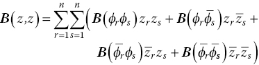
The total aerodynamic loads consist of contributions arising from the section motion, trailing‐edge flap rotation, and the penetration into a gusty field, as illustrated in Figure 4.4. The aerodynamic loads due to an arbitrary input time‐history are obtained through convolution against a kernel function. Since the assumption is of linear aerodynamics, the effects of the various influences on the aerodynamic forces and moments are added together to find the variation of the forces and moments in time for a given motion and gust. It follows that
where the dependence on time is not shown explicitly. The sub‐index i is used to denote the lift coefficient, ![]() , and pitch‐moment coefficient,
, and pitch‐moment coefficient, ![]() , whereas s, f and g indicate the contributions from the section motion, flat rotation, and gust perturbation, respectively. A schematic representation of the various contributions to the aerodynamic loads is shown in Figure 4.4.
, whereas s, f and g indicate the contributions from the section motion, flat rotation, and gust perturbation, respectively. A schematic representation of the various contributions to the aerodynamic loads is shown in Figure 4.4.


Figure 4.4 Schematic of a slender wing structure showing various contributions to the aerodynamic loads.
A brief description of each contribution to the total aerodynamic loads is summarised in the following three subsections. Note that, as is common in aerodynamics, the loads are formulated using non‐dimensional time, ![]() , which is also adopted for the time derivative,
, which is also adopted for the time derivative, ![]() . The subindex 0 will be used to indicate initial conditions.
. The subindex 0 will be used to indicate initial conditions.
Section Motion
The first term on the right‐hand side of Eq. (4.1) indicates the increment in the aerodynamic loads caused by a generic motion of the wing section. Each structural node of the beam stick model (see Section 4.2.3), has six degrees of freedom: three rotations and three translations. As the aerodynamic model here is two‐dimensional, the resulting motion of the wing section in the three‐dimensional space is projected onto the plane defining the wing cross section. Referring to Figure 4.4b, the motion of the wing section contributing to the aerodynamic loads consists of the vertical displacement of the structural beam model, denoted by h, and a rotation around the elastic axis, denoted by θ. This information is readily available from the solution of the structural problem.
We denote by α the effective angle of incidence of the wing section, which includes the freestream angle of attack, ![]() , and the wing torsional deformation, θ. Scale the vertical displacement, h, by the semi‐chord of the wing cross section,
, and the wing torsional deformation, θ. Scale the vertical displacement, h, by the semi‐chord of the wing cross section, ![]() . The resulting force and moment coefficients for any arbitrary section motion in pitch and plunge are formulated as
. The resulting force and moment coefficients for any arbitrary section motion in pitch and plunge are formulated as


The Wagner function, φw, accounts for the influence of the shed wake, and is known exactly in terms of Bessel functions. For a practical evaluation of the integral, the exponential approximation of Jones (1940) is used:
where the constants are ![]() ,
, ![]() ,
, ![]() and
and ![]() .
.
Trailing‐edge Flap Rotation
The second term on the right‐hand side of Eq. (4.1) represents the increment in the aerodynamic loads for any arbitrary trailing‐edge rotation, see Figure 4.4a. The build‐up in the loads not only depends on the instantaneous flap rotation but also on its time derivatives (velocity and acceleration). The relations between the control surface input, δ, and the load coefficients are
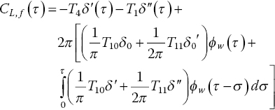

The coefficients T1, T4, T7, T8, T10 and T11 are geometric constants that depend on the size of the trailing‐edge flap relative to the chord of the wing section. The reader can find the full expressions in Da Ronch et al. (2014).
Atmospheric Gust
The last term on the right‐hand side of Eq. (4.1) describes the effect that atmospheric gusts and turbulence have on the build‐up of aerodynamic loads. For an arbitrary gust time‐history, the load coefficients are computed by the following relations:


where the gust intensity, wg, is normalised by the freestream speed. The integration uses the exponential approximation of the Küssner function
where the coefficients ![]() ,
, ![]() ,
, ![]() and
and ![]() are from Leishman (1994). Appropriate forms of wg to model realistic atmospheric gust and turbulence time‐histories are presented in some detail in Section 4.2.4.
are from Leishman (1994). Appropriate forms of wg to model realistic atmospheric gust and turbulence time‐histories are presented in some detail in Section 4.2.4.
4.2.3 Flexible–body Dynamics Model
For the structural model, the geometrically‐exact nonlinear beam equations are used (Hesse and Palacios 2012). Results are obtained using two‐noded displacement‐based elements. In a displacement‐based formulation, nonlinearities arising from large deformations are cubic terms, as opposed to an intrinsic description where they appear up to second order. The coupled flexible multibody nonlinear equations are expressed in the form

The subscripts s and r denote elastic and rigid‐body degrees of freedom, respectively. The terms Qgyr and Qstiff indicate, respectively, gyroscopic and elastic forces, whereas RF contains all external forces acting on the system, including aerodynamic contributions. More details of the structural modelling of multibody dynamics using finite elements can be found in Geradin and Cardona (2001).
Equation (4.10) is coupled with the linearised quaternion equations that propagate the orientation of the body frame with respect to the inertial frame.
4.2.4 Atmospheric Gust and Turbulence Models
In flight, aircraft regularly encounter atmospheric turbulence. For linear analysis, turbulence is regarded as a set of component velocities superimposed on a steady background flow. The aircraft experiences rapid changes in lift and moment forces, which cause rigid and flexible dynamic responses of the entire aircraft. These responses can cause passenger discomfort and introduce large loads on the structure and they must be accounted for during the design stage to ensure aircraft safety. The models used for the prediction of the aircraft response have to incorporate events that are perceived as discrete, usually described as ‘gusts’, as well as the phenomena described as continuous, in other words turbulence.
A concise summary of the mathematical models used to approximate discrete and continuous turbulent events is given next. The reader may find a more extensive review in Etkin (1981).
Discrete Deterministic Gusts
Discrete events are isolated encounters with steep gradients in the speed of air, which typically occur at the edges of thermals and downdrafts, in the wakes of structures or mountains, or at temperature inversions. Discrete gusts may also appear as rare extremes of turbulence in clouds, and so on, possibly associated with organised structures embedded in the otherwise random background. These organised extremes are not adequately allowed for in the usual Gaussian models of continuous random turbulence, and specialised discrete models should then be used.
The most common discrete gust model, which has evolved over the years from the isolated sharped‐edge gust function used in the earliest airworthiness assessments, is the ‘one‐minus‐cosine’ function:
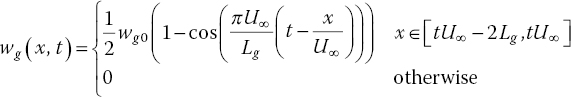
where wg0 is the gust intensity, Lg is the gust length, and x is the position of a point on the aircraft relative to an aircraft‐attached frame of reference (see Figure 4.5). The design gust velocity, wg0, varies with the gust length and the altitude and speed of flight (Hoblit 1988). In the simple case of Eq. (4.12), the gust intensity depends on one spatial coordinate, x, in addition to the time coordinate, t. The rate of change of the gust intensity at different points on the aircraft – say the main wing and tailplane – largely depends on two ratios (see Figure 4.5). The first ratio describes the relative size of the gust compared to the aircraft characteristic length. The second relates to the time it takes for the aircraft to fly over the gusty field. As these two ratios decrease, the dependence on the spatial coordinate becomes more and more apparent and should be modelled appropriately when simulating the aircraft response to relatively short gusts.


Figure 4.5 Discrete model of a one‐minus‐cosine gust.
Random Turbulence
Random turbulence is a chaotic motion of the air and is described by its statistical properties. The main statistical features that need to be considered are: stationarity, homogeneity, isotropy, time and distance scales, probability distributions, correlations and spectra. Atmospheric turbulence is a vector process in which the velocity vector is a random function of the position vector and of time. Because of the complexity introduced by this multi‐dimensionality, the description of turbulence and the associated input/response problems are often simplified, whether justified or not, to a one‐dimensional representation.
The engineering model of random turbulence at altitude has been developed over many years; see for example (Houbolt 1973). It is now widely accepted that it is satisfactory to treat atmospheric turbulence as frozen, homogeneous and isotropic in relatively large patches. The frozen‐field assumption, closely allied to Taylor’s hypothesis, is that turbulent velocities do not change during the time of passage of the airplane. This is a valid assumption in most cases. The Dryden and the von Kármán models are considered adequate engineering models to predict the correlation and spectra, with the weight of experimental evidence favouring the latter. Although there is much evidence that turbulence is not in fact a Gaussian process, with small and large values both occurring more frequently than in a normal distribution, the assumption that individual patches are Gaussian is widely used because of the great analytical advantage it offers.
A commonly used spectrum that matches experimental data is the von Kármán model. The power spectral density (PSD, in [m2/(s2 Hz)]) for the vertical direction, Φz, according to Military Specification MIL‐F‐8785C, is given by (Moorhouse and Woodcock 1982):

where ![]() is the scaled frequency (in [rad/m]), σz is the root mean square turbulence velocity (in [m/s]), Lz is the characteristic scale wavelength of the turbulence (in [m]), and
is the scaled frequency (in [rad/m]), σz is the root mean square turbulence velocity (in [m/s]), Lz is the characteristic scale wavelength of the turbulence (in [m]), and ![]() is the von Kármán constant. Figure 4.6 illustrates the PSD spectrum as function of the frequency. Whilst the system response in the frequency domain to a random turbulence can easily be calculated once the frequency‐response function is known, this approach is linear and does not permit nonlinear effects to be included in the analysis. An alternative approach is to generate a random turbulence time signal with the required spectral characteristics defined in Eq. (4.13), and solve the nonlinear system of equations in the time domain.
is the von Kármán constant. Figure 4.6 illustrates the PSD spectrum as function of the frequency. Whilst the system response in the frequency domain to a random turbulence can easily be calculated once the frequency‐response function is known, this approach is linear and does not permit nonlinear effects to be included in the analysis. An alternative approach is to generate a random turbulence time signal with the required spectral characteristics defined in Eq. (4.13), and solve the nonlinear system of equations in the time domain.
![Graph of gust vertical speed [m/s] over time with two waveforms for Simulink (solid) and VKTG (grayed).](http://images-20200215.ebookreading.net/13/1/1/9781118928684/9781118928684__advanced-uav-aerodynamics__9781118928684__images__c04f006a.gif)
![Graph of frequency [Hz] vs. PSD [m2/(s2 Hz)], with two frequency waves for Simulink (solid) and VKTG (grayed) and a descending curve for Von Karman.](http://images-20200215.ebookreading.net/13/1/1/9781118928684/9781118928684__advanced-uav-aerodynamics__9781118928684__images__c04f006b.gif)
Figure 4.6 Random vertical gust intensity using the von Kármán spectral representation (Military Specification: MIL‐F‐8785C; flight speed:  280 m/s; altitude:
  10,000 m; and turbulence intensity: ‘light,
  ’); the terms ‘Simulink’ and ‘VKTG’ denote, respectively, the Von Kármán Wind Turbulence Model block of MATLAB and the Von Kármán Turbulence Generator implementation.
A method to calculate the time‐domain response of a nonlinear aeroelastic model to random turbulence is as follows. First, take the Fourier transform of a unit variance band‐limited white noise signal, X(Ω), and pass it through a filter defined as the square root of the PSD spectrum in Eq. (4.13), Hz(Ω). Then calculate the output signal using the relation
Take the inverse Fourier transform of Wg(Ω) to obtain the random turbulence in the time domain, wg(t). This method, which applies a Fourier transform twice, is preferred over an alternative method that does not make use of the Fourier transform. More details may be found in Gianfrancesco (2014).
The method described above is implemented in an open source MATLAB toolbox called the Von Kármán Turbulence Generator (VKTG). The VKTG toolbox implements the mathematical representations of random turbulence defined in Military Specification MIL‐F‐8785C and Military Handbook MIL‐HDBK‐1797, allowing for the dependence of the root mean square turbulent velocity and turbulence length scale on aircraft mission parameters and weather conditions. As shown in Figure 4.6, at higher frequencies, the PSD of the VKTG model correlates more closely with the von Kármán spectrum of Eq. (4.13) than an off‐the‐shelf MATLAB/SIMULINK model. Note that the VKTG toolbox accompanying this chapter is also available online.2
4.2.5 Numerical Implementation
With the previous sections as background, the coupled dynamics of a flexible flying aircraft encountering atmospheric gusts and turbulence requires a careful integration of each single discipline within a comprehensive simulation environment. It is generally possible to recast the complete system of equations in state‐space form, this being convenient for the derivation of the reduced‐order model, as discussed in Section 4.3.
4.3 Coupled Reduced‐order Models
The numerical solution of a nonlinear system in the time domain requires the integration of the differential equations that govern its dynamics. Numerical schemes are often referred to as being explicit or implicit. For the conditional stability of explicit methods, a small time step is required to solve the small timescales that are always present in spatially detailed models but that are not needed in our analysis. Implicit methods, which are more complex to program and require more computational effort in each solution step, are therefore preferred because they allow for longer time steps. As most of the computational methods to solve nonlinear systems were developed for first‐order ordinary differential equations (ODEs), it is convenient to reformulate the coupled system as a system of first‐order ODEs.
Let us consider as a starting point the nonlinear system
where the nonlinear operator ![]() depends on the specific formulation used. For brevity,
depends on the specific formulation used. For brevity, ![]() denotes the time derivative, d(•)/dt. Consider the coupled system partitioned as follows
denotes the time derivative, d(•)/dt. Consider the coupled system partitioned as follows
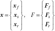
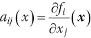
where the subindices f, s and r indicate, respectively, the fluid, structural, and rigid‐body (flight dynamics) degrees of freedom. Denote by u the vector of manipulable inputs, generally used for control purposes, and by d the vector of exogenous disturbances perturbing the system. Indicate the ith component of F by fi. If the components of F are differentiable at ![]() , define the Jacobian matrix
, define the Jacobian matrix ![]() as
as
or in matrix form as
for any constant vector of manipulable inputs and exogenous disturbances, ũ and ![]() , respectively.
, respectively.
4.3.1 Approaches to Model Reduction
The difficulty with Eq. (4.15) is the size of the computational model which, for realistic applications, may include ![]() to
to ![]() degrees of freedom. To accelerate the time‐domain analysis and allow design of a low‐order control system, a reduced‐order model of Eq. (4.15) is often needed in practice.
degrees of freedom. To accelerate the time‐domain analysis and allow design of a low‐order control system, a reduced‐order model of Eq. (4.15) is often needed in practice.
Two approaches to reduce the size of a system exist. The first is based on system identification techniques that attempt to replace the original large computational model, which is treated as a ‘black box’, with a system of smaller size. Often the model structure is simplified, allowing for some forms of nonlinearity to be included. The advantages are the easiness of the numerical implementation and the availability of various techniques (Volterra series, indicial functions, surrogate models, and so on). The disadvantages are the lack of robustness of the system parameters and the limited validity and certainty for conditions outside those used to generate the model. More details may be found in Ghoreyshi et al. (2013) and Da Ronch et al. (2011).
The second approach involves manipulation of the governing equations in Eq. (4.15). The advantages are the ability to retain nonlinear effects in a smaller system and that the system validity depends on the assumptions made to derive the model. The disadvantage is the added complexity in the model implementation. Two well‐established reduced‐order models for application in unsteady aerodynamics and aeroelasticity are based on the harmonic balance method (Da Ronch et al. 2013a) and nonlinear model projection (Da Ronch et al. 2012), respectively.
The approach to model reduction first presented in Da Ronch et al. (2012) and thereafter applied extensively to various problems and test cases (Da Ronch et al. 2013b, 2014, 2013c; Tantaroudas et al. 2014; Timme et al. 2013), is discussed in more detail in the following sections. The approach is based on the manipulation of the governing equations and consists of a systematic procedure to generate both linear and nonlinear reduced‐order models, independently of the mathematical formulation used in the coupled system. The approach also satisfies the properties outlined in Section 4.1.1.
4.3.2 Stability Analysis
Neglect first the explicit dependence of the system in Eq. (4.15) on the time variable, and consider a constant vector of manipulable inputs and exogenous disturbances, ũ and ![]() . Here, for simplicity,
. Here, for simplicity, ![]() is assumed. An equilibrium point,
is assumed. An equilibrium point, ![]() , satisfies the relation
, satisfies the relation
The stability of the system in the neighbourhood of the equilibrium point, ![]() , is studied through an eigenvalue analysis. Define a small increment with respect to the equilibrium point,
, is studied through an eigenvalue analysis. Define a small increment with respect to the equilibrium point, ![]() . The linearised homogeneous system around the equilibrium point,
. The linearised homogeneous system around the equilibrium point, ![]() , takes the form
, takes the form
where A is the Jacobian matrix, Eq. (4.18). Let us consider a solution of Eq. (4.20) in the exponential form
where λ is a constant scalar and ϕ is a constant n‐dimensional vector. The right and left eigenvalue problems associated with this ansatz, after substituting Eq. (4.21) into Eq. (4.20), are
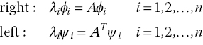
For large computational models, the solution of the above eigenvalue problems using off‐the‐shelf algorithms is unfeasible. Because the subject is out of the scope of this chapter, the interested reader is referred to Badcock et al. (2011). Here, let us assume an appropriate eigenvalue solver is available for solving the right and left problems.
It is convenient to normalise the eigenvectors to satisfy the biorthonormality conditions. This will be of great benefit when deriving the reduced‐order model.

so that the relation holds
where δij is the Kronecker delta and the operator (•)H indicates the Hermitian transpose: the transpose of the complex conjugate.
4.3.3 Model Projection
An attempt to solve Eq. (4.15) may not only require large computational resources but it is also not well suited to the design of a low‐order control system. The idea of transforming the above set of n simultaneous nonlinear equations into one that lends itself to an easier solution arises naturally. As is common in structural dynamics, a transformation of coordinates defined in terms of the n orthonormal modal vectors ϕ1, ϕ2, …, ϕn, is an efficient choice (Meirovitch 1990). Let define w in the form of a linear combination of modal vectors
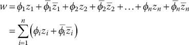
where the over‐bar sign ![]() indicates the conjugate. It is worth noting that the solution of the eigenvalue problems in Eq. (4.22) provides the eigenvalues and the associated eigenvectors of the coupled system, describing the interactions between the fluid, structural, and flight mechanics fields. It follows that the transformation of coordinates defined in Eq. (4.25) generalises the well‐known approach used in structural dynamics for coupled problems. The approach retains the high efficiency of the basis functions, created using the coupled modal vectors, to allow fast convergence even for non‐homogeneous cases.
indicates the conjugate. It is worth noting that the solution of the eigenvalue problems in Eq. (4.22) provides the eigenvalues and the associated eigenvectors of the coupled system, describing the interactions between the fluid, structural, and flight mechanics fields. It follows that the transformation of coordinates defined in Eq. (4.25) generalises the well‐known approach used in structural dynamics for coupled problems. The approach retains the high efficiency of the basis functions, created using the coupled modal vectors, to allow fast convergence even for non‐homogeneous cases.
Modal analysis in structural dynamics is a powerful tool to ensure good approximations of the ‘exact’ solution obtained through time integration of Eq. (4.15) using a relatively small number of modal vectors. This property holds for the coupled model presented herein. Because the structural response is generally well represented by the low‐frequency normal modes, it is not unexpected that a small basis of coupled modeshapes dominated by the motion of the structure is critical for the aeroelastic response.
To achieve a significant reduction in the system size, a small basis of biorthonormal coupled eigenvectors and associated eigenvalues representative of the system dynamics defined in Eq. (4.15) should be identified. Let us collect m coupled eigensolutions in the modal matrices of the right and left eigenvectors

where the diagonal matrix Λ has dimension ![]() and the matrices Φ and Ψ have dimension
and the matrices Φ and Ψ have dimension ![]() .
.
Truncate the linear combination in Eq. (4.25) to include ![]() terms
terms

where the columns ϕi of the ![]() matrix Φ span the subspace within which the system motion is now restricted. The transformation of coordinates relates the state‐space vector of the large‐order coupled model,
matrix Φ span the subspace within which the system motion is now restricted. The transformation of coordinates relates the state‐space vector of the large‐order coupled model, ![]() , with the stat‐ space vector of the reduced‐order coupled model,
, with the stat‐ space vector of the reduced‐order coupled model, ![]() . To ensure convergence of the results, it is common to start with a small basis of coupled eigenvectors, then expanding this until the results have fully converged. A study of the model convergence is described in Section 4.3.6.
. To ensure convergence of the results, it is common to start with a small basis of coupled eigenvectors, then expanding this until the results have fully converged. A study of the model convergence is described in Section 4.3.6.
4.3.4 Linear Reduced Order Model
Let us start with the linearised model of Eq. (4.15). For simplicity, consider a constant equilibrium point, ![]() , when no control inputs and disturbances are acting on the system,
, when no control inputs and disturbances are acting on the system, ![]() and
and ![]() , respectively. Note that u and d are independent of the equilibrium point, whereas
, respectively. Note that u and d are independent of the equilibrium point, whereas ![]() depends on both control and disturbance vectors. It follows that the linearised system has the form
depends on both control and disturbance vectors. It follows that the linearised system has the form
As the above linearised system still retains the size of the coupled nonlinear system, the transformation of coordinates may be used to derive a linear reduced‐order model. First, substitute Eq. (4.27) into Eq. (4.28), then pre‐multiply each term by the Hermitian transpose of the left modal matrix, ΨH. Recalling the biorthonormal properties in Eq. (4.23) and (4.24), it follows that a linear reduced‐order model has the form
where ![]() and
and ![]() . Solving the linear reduced‐order model in Eq. (4.29) offers two important computational advantages. The first is that the system consists of a set of independent (uncoupled) equations that exploit the biorthonormal properties of the modal basis which makes the system much easier to solve. The second advantage is that we have achieved a reduction in the system size,
. Solving the linear reduced‐order model in Eq. (4.29) offers two important computational advantages. The first is that the system consists of a set of independent (uncoupled) equations that exploit the biorthonormal properties of the modal basis which makes the system much easier to solve. The second advantage is that we have achieved a reduction in the system size, ![]() , by exploiting very efficient basis functions. As a result, a very efficient model of small size can be used to predict the time‐domain response.
, by exploiting very efficient basis functions. As a result, a very efficient model of small size can be used to predict the time‐domain response.
4.3.5 Nonlinear Reduced‐order Model
Next, let us consider a way to incorporate nonlinear effects in the reduced‐order model. There are two basic requisites to meet. The first relates to the difficulty of the implementation and the cost of model generation, which should be as low as possible to facilitate its exploitation. The second is that it is desirable to have a formulation that is independent of the equations used to create the model, so that the approach to nonlinear model reduction is systematic and applicable, in principle, to any coupled system. The method presented in Da Ronch et al. (2012) meets both requirements.
An approach to systematically derive nonlinear reduced‐order models indeed exists. Expand the nonlinear system in Eq. (4.15) in a Taylor series retaining terms up to third order in the perturbation. It follows that
where the additional terms, compared to Eq. (4.28), indicate the second‐ and third‐order Jacobian operators. It is immediate seen that the operators B and C are, respectively, bi‐linear and tri‐linear with respect to the arguments and are analytically obtained as

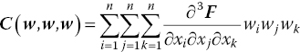
The difficulty with substituting the transformation of coordinates, Eq. (4.27), into Eq. (4.30) is the treatment of the quadratic and cubic terms, B and C, respectively. After some manipulations and recalling the linearity of the high‐order operators, a relatively simple relation is found. For brevity, the form of the quadratic term is reported
The interested reader is invited to refer to Da Ronch et al. (2012) for the relation for the cubic term. Here it is sufficient to note that the double sum may be further simplified by taking advantage of the bi‐linearity of B, that is, ![]() , reducing the total number of calculations required to compute B(z, z).
, reducing the total number of calculations required to compute B(z, z).
The final step, as already done for the linear reduced‐order model, is to pre‐multiply each term of Eq. (4.30), once expressed as a function of z and not of w, by the Hermitian transpose of the left modal matrix, ΨH. The nonlinear reduced‐order model then has the form
where fnln(z) contains the nonlinear terms of the quadratic and cubic operators.
Numerical Implementation
A final note on the numerical approach used to calculate the higher‐order terms of the nonlinear reduced‐order model. It is possible to calculate all the contributions without having to resort to complex arithmetic or calculating all the second‐ and third‐order partial derivatives analytically. Because it is only their action on vectors that is required, matrix‐free products may be used. The evaluation of the finite differences suffers from the truncation error for values of the step size that are too large, and from the rounding error for values that are too small. The latter effect is more significant for the coefficients that include a third Jacobian product. In cases where convergence of the finite differences for various step sizes is not found, it is possible to resort to the MATLAB libraries supporting extended‐order arithmetics; see Da Ronch et al. (2013c).
The approach to the generation of the reduced‐order model detailed above leads to the set of equations described next. The equations of the reduced‐order model are independent of the specific formulation used for the full order model, and are always expressed in a state‐space form.
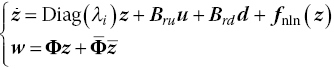
The dynamics of the nonlinear reduced‐order model in Eq. (4.35) are given in terms of a complex‐valued state vector, z, which is of small size. The output equation defines how the physical degrees of freedom of the original full‐order model can be retrieved if necessary. The control inputs and disturbances are in the vectors u and d, respectively. For the linear aerodynamics described in Section 4.2.2, it is apparent that the control surface rotation, angular velocity and acceleration are treated as commanded inputs. Keeping these quantities as separate inputs is not convenient, as the three quantities are all linked by a time integration/derivation relationship. Referring to Da Ronch et al. (2014), it is possible to see that the actual commanded control input is the angular acceleration of the control surface, and that the angular velocity and rotation are easily deduced by numerical time integration.
4.3.6 Aircraft Test Case Gust Response
Having presented a set of mathematical models for the description of flexible aircraft dynamics and a model‐reduction strategy to reduce costs, a demonstration of these tools is now performed for the flexible unmanned aircraft test case of Section 4.2.1. The freestream conditions are ![]() 59 m/s,
59 m/s, ![]() 4° and
4° and ![]() 0.0789 kg/m3. In flight, the aircraft exhibits large wing deformations. The deformed shape is computed from a static aeroelastic solution and taken as the equilibrium point for the reduced model generation. The coupled large‐order model, hereafter referred to as the full‐order model (FOM), consists of 540 degrees of freedom, 324 associated with the structural model and 216 with the aerodynamic model.
0.0789 kg/m3. In flight, the aircraft exhibits large wing deformations. The deformed shape is computed from a static aeroelastic solution and taken as the equilibrium point for the reduced model generation. The coupled large‐order model, hereafter referred to as the full‐order model (FOM), consists of 540 degrees of freedom, 324 associated with the structural model and 216 with the aerodynamic model.
First, the right and left eigenvalue problems are solved around the static aeroelastic deformed shape. As the identification of an adequate basis for the model projection is critical for the analysis, a preliminary study is done to ensure convergence by increasing the size of the modal basis, Eq. (4.26). A reasonable approach is to initially include a number of coupled modes that are dominated by the structural response. These modes are associated with the normal modes of the structure when the surrounding fluid is removed. In addition to this clear choice, the inclusion of the so called ‘gust modes’ is needed to enrich the modal basis for gust load prediction. In linear aerodynamics, these modes are easily identified, being related to the smallest Küssner constant, ![]() . The eigenvalues of the ‘gust modes’ are
. The eigenvalues of the ‘gust modes’ are ![]() (in [Hz]). Tests to ensure convergence of the modal basis were done using up to eight coupled eigenvalues, as summarised in Table 4.2. The first five coupled modes are mainly dominated by the structural response and are traced for these flight conditions from the corresponding normal modes of the structure. The remaining modes are ‘gust modes’ and provide the mechanisms to describe the influence of an atmospheric gust on the structural response. The variation of the frequencies of the coupled modeshapes with respect to the freestream speed is shown in Figure 4.7.
(in [Hz]). Tests to ensure convergence of the modal basis were done using up to eight coupled eigenvalues, as summarised in Table 4.2. The first five coupled modes are mainly dominated by the structural response and are traced for these flight conditions from the corresponding normal modes of the structure. The remaining modes are ‘gust modes’ and provide the mechanisms to describe the influence of an atmospheric gust on the structural response. The variation of the frequencies of the coupled modeshapes with respect to the freestream speed is shown in Figure 4.7.
Table 4.2 Basis of coupled eigenvalues used for the model projection; see Eq. (4.26).
| Mode number | Modeshape | Real part | Imaginary part |
| Hz | Hz | ||
| 1 | First bending |
–8.82 |
±1.97 |
| 2 | Second bending |
–8.04 |
±9.81 |
| 3 | First torsion |
–1.71 |
±1.45 |
| 4 | Third bending |
–7.03 |
±2.17 |
| 5 | Fourth bending |
–6.04 |
±4.19 |
| 6 | Gust mode | – 9.90 | 0.00 |
| 7 | Gust mode |
–1.01 |
0.00 |
| 8 | Gust mode |
–1.01 |
0.00 |

Figure 4.7 Dependence on freestream speed of coupled aeroelastic frequencies for: (a) structurally‐dominated modeshapes and (b) gust modeshapes.
The convergence of a linear reduced‐order model for increasing size of the modal basis is shown in Figure 4.8. The open‐loop response is computed for a random turbulence with statistical properties defined by the von Kármán spectrum. The reduced‐order model predictions are compared with those of the original full‐order model, with dimension 540 degrees of freedom. Good agreement is observed, with as low as eight coupled modes for the reduced‐order model. To emphasise when a model is nonlinear, ‘N’ is appended to the shorthand notation.

Figure 4.8 Gust response of the aircraft test case: (a) convergence for increasing number of coupled modes and (b) vertical gust intensity normalised by  . Military specification: MIL‐F‐8785C.
  59 m/s,
  4°,
4°,  0.0789 kg/m3 and turbulence intensity: ‘severe
  ’. FOM, full‐order model; ROM, reduced order model.
Next, the reduced‐order model is demonstrated for the efficient search of the worst‐case gust. The search is conducted for the one‐minus‐cosine gust family considering gust wavelengths between 0 and 776 aircraft mean aerodynamic chords (with a step size of 9.7). A strong gust intensity, 14% of the freestream speed, causes large wing structural deformations. In addition to the linear reduced model above, a nonlinear reduced‐order model was generated with the same modes but including terms up to second order. The inclusion of higher‐order terms did not modify the convergence properties of the model. The search was performed using both the full‐ and reduced‐order models and 80 calculations were performed in total. Figure 4.9 illustrates the largest upward and downward structural deflections of the wing tip for various gust wavelengths. These are reported along the horizontal axis. The worst‐case gust causing the largest structural deformation is seen to have a 4 s duration, corresponding to a length of 197 mean aerodynamic chords at the flying speed of 59 m/s. The dynamic response to the worst‐case gust is compared for linearised and nonlinear models, and also for the full‐ and reduced‐order models. Deformations of 9 m are considered large, because the wing span is 17.75 m, and it is not unexpected in this case that the linearised (full and reduced) models over‐predict the deformations. The computational cost to obtain the gust profiles in Figure 4.9 with the reduced models was a fraction of that needed for the original full model: for the linear case, the reduced model was 10 times as fast; for the nonlinear case, an increased performance of about 30 times was recorded. These indicative values are expected to increase considerably as the size of the original model increases (Da Ronch et al. 2013c), demonstrating the practical use and advantage of our approach to model reduction.

Figure 4.9 Worst‐case gust search for the one‐minus‐cosine gust family: (a) profile of largest structural deflections at the wing tip and (b) dynamic response for the tuned worst‐case gust. NFOM, nonlinear full‐order model; FOM, full‐order model; NROM, nonlinear reduced‐order model; ROM, reduced‐order model.
To conclude, it is demonstrated through application to a realistic HALE test case that the reduced‐order models significantly reduce the computational cost for parametric worst‐case gust searches. Section 4.4.3 will also show that the reduced‐order models are adequate for a variety of control designs for gust load alleviation.
4.4 Control System Design
Previous work by the authors has considered the systematic generation of nonlinear reduced models that not only capture the system nonlinearities but also are parameterised with respect to flow conditions such as freestream speed and density (Da Ronch et al. 2012, 2013b; Papatheou et al. 2013). The reduced models were used for ![]() control design for gust load alleviation. In general, the
control design for gust load alleviation. In general, the ![]() control provides strong disturbance rejection but, in principle, a controller that can adapt during changes of the flow conditions, such as airspeed or density, is desired. Recently, an adaptive controller was found efficient for gust load alleviation for a flexible wing (Tantaroudas et al. 2014). That study, in addition to a comparison of control design performance, emphasised the fact that inherently different control methodologies, from robust controllers to nonlinear adaptive controllers, can be designed based on the very same nonlinear reduced‐order model in Eq. (4.35).
control provides strong disturbance rejection but, in principle, a controller that can adapt during changes of the flow conditions, such as airspeed or density, is desired. Recently, an adaptive controller was found efficient for gust load alleviation for a flexible wing (Tantaroudas et al. 2014). That study, in addition to a comparison of control design performance, emphasised the fact that inherently different control methodologies, from robust controllers to nonlinear adaptive controllers, can be designed based on the very same nonlinear reduced‐order model in Eq. (4.35).
This section continues with an overview of the theory behind two control strategies: ![]() synthesis in Section 4.4.1 and model reference adaptive control in Section 4.4.2. Finally, Section 4.4.3 presents a comparison of the two control strategies in gust load alleviation in the aircraft test case.
synthesis in Section 4.4.1 and model reference adaptive control in Section 4.4.2. Finally, Section 4.4.3 presents a comparison of the two control strategies in gust load alleviation in the aircraft test case.
4.4.1  Synthesis
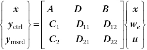
Starting from Eq. (4.35), a manipulation is needed to recast the system of equations for ![]() control synthesis. First, observe that the equations of the reduced‐order model dynamics are complex‐valued and this is incompatible for control design. The system of equations is easily recast in real form, splitting the real and imaginary parts into separate equations and doubling its original dimension. Second, recall that for linear aerodynamics, the rotation δ, angular velocity δ′ and acceleration δ′′ of a control surface contribute to the build‐up of the aerodynamic loads. As an interdependency exists between these three quantities, the actual commanded input is chosen to be the control surface angular acceleration, from which the deflection and angular velocity can be calculated numerically. It follows that it is more convenient to perform control design synthesis around the following set of equations rather than Eq. (4.35):
control synthesis. First, observe that the equations of the reduced‐order model dynamics are complex‐valued and this is incompatible for control design. The system of equations is easily recast in real form, splitting the real and imaginary parts into separate equations and doubling its original dimension. Second, recall that for linear aerodynamics, the rotation δ, angular velocity δ′ and acceleration δ′′ of a control surface contribute to the build‐up of the aerodynamic loads. As an interdependency exists between these three quantities, the actual commanded input is chosen to be the control surface angular acceleration, from which the deflection and angular velocity can be calculated numerically. It follows that it is more convenient to perform control design synthesis around the following set of equations rather than Eq. (4.35):

where ![]() , with wd indicating an artificial disturbance used in tuning the variables of the control synthesis, and
, with wd indicating an artificial disturbance used in tuning the variables of the control synthesis, and ![]() . The output is distinguished by what the controller is aiming to control, yctrl, and what the controller has information about, ymsrd.
. The output is distinguished by what the controller is aiming to control, yctrl, and what the controller has information about, ymsrd.
The ![]() control problem with additional input‐shaping techniques for control tuning purposes for the classical
control problem with additional input‐shaping techniques for control tuning purposes for the classical ![]() problem formulation is written as follows (Zhou and Doyle 1998),
problem formulation is written as follows (Zhou and Doyle 1998),
The resulting controller has the linear form
where K(s) is the ![]() controller transfer function in the Laplace domain. The aim is to minimise the transfer of the disturbance signal from d to yctrl by creating a controller that uses information from ymsrd to change the input u. This can be written as
controller transfer function in the Laplace domain. The aim is to minimise the transfer of the disturbance signal from d to yctrl by creating a controller that uses information from ymsrd to change the input u. This can be written as

where γ represents the ratio of the maximum output energy to the maximum input energy.
The problem is expanded to include a weight on inputs, Kc, which carries over to an additional element on controlled output and a weight on measurement noise, Kd, which carries over to an additional element on measured output. The ![]() control is derived on the basis of the linearised model and is applied directly to the nonlinear full‐order model by using the reduced matrices from the nonlinear model order‐reduction framework.
control is derived on the basis of the linearised model and is applied directly to the nonlinear full‐order model by using the reduced matrices from the nonlinear model order‐reduction framework.
4.4.2 Model Reference Adaptive Control
Assume the nonlinear reduced‐order model in the form of Eq. (4.35), and consider an ideal model reference in the form
Matrix Am is a stable Hurwitz matrix that meets the desired properties of the reference system. This could mean eigenvalues with increased damping compared to the actual aeroelastic system. Matrix Bm is user defined and describes the influence of the control inputs on the states of the reference model. The states of the reference model due to the increased damping in matrix Am will decay to zero faster under the same disturbances or flap actuation while their magnitude will be in general smaller as well. The physical displacements of the system can be retrieved using the output equation.
The goal is to find a dynamic control input, u, related to the flap actuation that satisfies the condition ![]() . The exact control feedback for the model matching conditions is defined as
. The exact control feedback for the model matching conditions is defined as
where r is a reference signal applied to both systems, as shown in Figure 4.10, representing in our case the flap angle, and ![]() are the exact gains acting on the states and control input to match the two models. Substituting Eq. (4.41) in Eq. (4.36) and satisfying the model matching conditions yields
are the exact gains acting on the states and control input to match the two models. Substituting Eq. (4.41) in Eq. (4.36) and satisfying the model matching conditions yields


Figure 4.10 Block diagram of a nonlinear adaptive control algorithm.
Since A and Bc are considered to be unknown to the controller, the values of ![]() in Eq. (4.41) are also unknown at the initial time and the actual control signal applied at the current time‐step is defined as
in Eq. (4.41) are also unknown at the initial time and the actual control signal applied at the current time‐step is defined as
K x and Kr in Eq. (4.43) are dynamic gains that need to be solved and at the end will be required to converge to the values that provide a solution to Eq. (4.42).
However, in adaptive control systems there is a major uncertainty about the convergence of the adaptive gains, even in deterministic ideal situations. In the presence of stochastic disturbances, this issue becomes even more challenging and complicated and this topic has remained open for many years in the field of nonlinear adaptive control design. There are many cases where the adaptive gains converge to values that are different to the actual analytical pre‐calculated ideal gains, even without the presence of disturbances. Recently, Barkana (2005) showed that in cases where the adaptive gains do not reach the unique solution that the preliminary design suggests, it is not because there is something wrong with the control design. This is because the adaptive controller only needs a specific set of gains that correspond to a particular input command, rather than the unique solution of gains for all inputs that an exact design suggests.
The closed‐loop dynamics of the nonlinear reduced model at this point may be expressed as
Let ![]() and
and ![]() . The estimation error between the instantaneous and the ideal gains is defined as
. The estimation error between the instantaneous and the ideal gains is defined as
with ![]() and
and ![]() . Now define
. Now define ![]() . In this case, the closed‐loop system dynamics in Eq. (4.44) are expressed as
. In this case, the closed‐loop system dynamics in Eq. (4.44) are expressed as
For the purpose of the stability proof of the closed‐loop system one needs to define the error dynamics between the two systems (Barkana 2013).
The derivative of this expresses the rate of change between the two systems and can be written as

At this point, the Lyapunov equation needs to be solved for the reference model because its solution will be part of the steady part of the Lyapunov candidate function that we define and that will lead to the stability proof of the nonlinear reduced model (Ioannou and Sun 1996).
where in Eq. (4.49) Q is a semi‐definite positive user‐defined matrix. A scalar quadratic Lyapunov function V in e and ![]() may be defined, such that the system becomes asymptotically stable by satisfying
may be defined, such that the system becomes asymptotically stable by satisfying ![]() . Its time derivative is semi‐definite negative
. Its time derivative is semi‐definite negative ![]() Ioannou and Sun (1996). This function will provide insight on the selection of the parameter update law of the time‐varying gains in Eq. (4.43). The Lyapunov function
Ioannou and Sun (1996). This function will provide insight on the selection of the parameter update law of the time‐varying gains in Eq. (4.43). The Lyapunov function
is considered, where ![]() is the solution of the algebraic Lyapunov equation (4.49) for a particular selection of Q while
is the solution of the algebraic Lyapunov equation (4.49) for a particular selection of Q while ![]() is a user‐defined semi‐definite positive matrix. Note that the positiveness of the above Lyapunov function is guaranteed only if the system under examination is a minimum‐phase system, which is enforced in the reduced‐order model generation. Differentiating the above equation with respect to time yields
is a user‐defined semi‐definite positive matrix. Note that the positiveness of the above Lyapunov function is guaranteed only if the system under examination is a minimum‐phase system, which is enforced in the reduced‐order model generation. Differentiating the above equation with respect to time yields
By substitution of the error dynamics and by using Eq. (4.49), Eq. (4.51) is expanded as follows
From thus, one can determine the adaptation parameter to satisfy the semi‐definite negativeness of the derivative of the Lyapunov function as
which leads to
The term ![]() in Eq. (4.54) is negative‐definite with respect to e and this is enforced by the semi‐definitive positive matrix Q. The derivative of the Lyapunov function remains negative definite in both x(t) and e(t) if additionally the second term in Eq. (4.54) is not too large, or alternatively if the following inequality is satisfied (Torres and Mehiel 2006):
in Eq. (4.54) is negative‐definite with respect to e and this is enforced by the semi‐definitive positive matrix Q. The derivative of the Lyapunov function remains negative definite in both x(t) and e(t) if additionally the second term in Eq. (4.54) is not too large, or alternatively if the following inequality is satisfied (Torres and Mehiel 2006):

However, it is impossible to come up with a general mathematical proof that ensures the stability of the nonlinear adaptive control scheme of flexible aircraft for all types of nonlinearities. Instead, the efficiency of the control design is demonstrated on the nonlinear system for realistic amplitudes of external disturbances. The dynamic time‐varying gains in Eq. (4.43) are updated by the adaptive law so that the time derivative of the Lyapunov function decreases along the error dynamic trajectories as in Eq. (4.54). By using Barbalat’s lemma this translates in boundness of the error dynamics with respect to the time evolution, and as a result the model‐matching conditions are satisfied.
In general, this control approach is limited to minimum phase systems. Thus, when applied in unstable non‐minimum phase systems, unstable zero‐pole cancellation may occur and the error between the two assumed models slowly diverges to infinity. However, a simple feedback based on the Bass–Gura formula (Ogata 2010) can be applied to the reduced‐order model to place any unstable zeros in the left half plane. The implementation of the computational algorithm is summarised in the block diagram shown in Figure 4.10.
4.4.3 Aircraft Test Case Gust‐load Alleviation
H∞ Synthesis
The design of a controller for load alleviation was performed on the linear reduced model considering the tuned worst‐case gust. The good performance of the controller in suppressing the vibrations of the linear model induced by the worst‐case gust is not unexpected, as the controller was designed specifically for that scenario. However, its performance will be shown on the nonlinear full model. The question addressed in this section is whether good alleviation can be achieved for a different shape of the gust, but using the same controller. The responses shown in Figure 4.11 are for the discrete worst‐case gust and for a continuous‐gust model based on the von Kármán spectrum. The aeroelastic vibrations of the closed‐loop system are significantly reduced when compared to the open‐loop response. However, the performance of the optimal robust controller is seen to degrade when applied to the nonlinear system for very strong stochastic disturbances.


Figure 4.11 Gust‐load alleviation response using the  controller compared to the open‐loop response: (a) worst‐case one‐minus‐cosine gust from Figure 4.9; (b) von Kármán turbulence model. NFOM, nonlinear full‐order model.
The efficiency of the optimal control approach using the reduced models for gust‐load alleviation can be demonstrated in a case with noticeable differences between the linear and nonlinear full‐order models; see Figure 4.9. However, the performance of the optimal robust controller is reduced when applied to the nonlinear system for very strong stochastic disturbances.
Model Reference Adaptive Controller
The nonlinear reduced model was implemented to simplify and speed up the calculation of the adaptive model reference control framework. The computed control surface deflection was applied to the nonlinear full‐order model, which is under external disturbances. The selection of the reference model is of critical importance; a bad choice could potentially lead the flap to undergo unrealistic rotations. In this case, a reference model was created with additional damping added to the first bending and torsional modes. As a result, the aeroelastic vibrations of the reference system die out more quickly than those of the plant to be controlled. The eigenvalues of the linearised reference system are summarised in the Table 4.3, which should be comprated to Table 4.2 for the uncontrolled system. Note that damping is added to the first five complex conjugate eigenvalues. The eigenvalues and a comparison of the plant model and the selected reference model for the worst‐case gust are shown in Figure 4.12.
Table 4.3 Eigenvalues of the reference model.
| Mode number | Real part | Imaginary part |
| 1 |
–9.53 |
±2.01 |
| 2 |
–8.53 |
±1.02 |
| 3 |
–1.71 |
±2.79 |
| 4 |
–5.73 |
±4.74 |
| 5 |
–1.21 |
±6.55 |
| 6 | –9.90 | 0.00 |
| 7 |
–1.01 |
0.00 |
| 8 |
–1.01 |
0.00 |

Figure 4.12 Ideal reference model for the MRAC controller design compared to the open‐loop response for: (a) worst‐case one‐minus‐cosine gust from Figure 4.9; (b) von Kármán turbulence model; (c) eigenvalues of the system to be controlled and the reference system.
The selection of the semi‐definite‐positive matrix Q that provides a solution to the Lyapunov equation given a stable Hurwitz matrix of a reference model Am is also critical. In this case, Q was chosen to be a diagonal matrix with elements ![]() . As shown in Eq. (4.53), the selection of the reference model will affect how e(t) will evolve during the time integration, which is part of the adaptation parameter. The reference model in that case needs to be stable so that the error decreases asymptotically. Finally, observe that the adaptation parameter is affected by P and, as a result, by matrices Q and Γ.
. As shown in Eq. (4.53), the selection of the reference model will affect how e(t) will evolve during the time integration, which is part of the adaptation parameter. The reference model in that case needs to be stable so that the error decreases asymptotically. Finally, observe that the adaptation parameter is affected by P and, as a result, by matrices Q and Γ.
The effect of the adaptation matrix Γ is therefore investigated for the performance of the closed‐loop system. The discrete selection of the semi‐definite‐positive matrix Γ is shown in Table 4.4 for both discrete and continuous gust‐load alleviation.
Table 4.4 Adaptation parameter selection.
| Discrete gust case | Continuous gust case | |
| Γ | 0.01Q | 0.01Q |
| Γ | 0.10Q | 0.10Q |
| Γ | 1.00Q | 1.00Q |
The derived controller based on the reduced model is directly applied to the full‐order nonlinear aeroelastic system. The wing‐tip vertical displacements for different adaptation rates for the worse‐case one‐minus‐cosine gust and for a continuous gust are shown in Figure 4.13.
Figure 4.13 Gust‐load alleviation response using the MRAC controller for various adaptation gains compared to the open‐loop response for: (a) worst‐case one‐minus‐cosine gust from Figure 4.9; (b) von Kármán turbulence model. NFOM, nonlinear full‐order model.
The results show a significant reduction of the wing‐tip deflections for the closed‐loop system for both linear and nonlinear cases, with realistic flap deflections in all cases. It can be seen that for the particular selection of the semi‐definite‐positive matrix Q, a larger adaptation gain Γ is required during the fluid–structure–gust interaction to alleviate the disturbances. A further increase of the adaptation gain may lead to a non‐realistic flap rotation with a flap angle of over 15°, which is a common constraint for the flap maximum rotation. Therefore, very large adaptation rates are not recommended, because the flap might overshoot during the fluid–structure–gust interaction.
Control Design Comparison
Both control designs were found adequate for gust‐load alleviation of a very flexible aircraft. However, a ‘good’ controller not only guaranteed that the closed‐loop structural deformations are smaller than those of its open‐loop counterpart, but also that this is achieved with a realistic, optimal and minimum control effort. The performance of the ![]() and MRAC controllers for the discrete one‐minus‐cosine gust is reported in Table 4.5. It is found that the adaptive control methodology achieves a better performance in reducing wing‐tip deflection than the
and MRAC controllers for the discrete one‐minus‐cosine gust is reported in Table 4.5. It is found that the adaptive control methodology achieves a better performance in reducing wing‐tip deflection than the ![]() control strategy, and the performance in gust‐load alleviation increases for increasing adaptation rates. The reduction in wing‐tip deflection is also achieved with a smaller control effort.
control strategy, and the performance in gust‐load alleviation increases for increasing adaptation rates. The reduction in wing‐tip deflection is also achieved with a smaller control effort.
Table 4.5 Comparison of control performance for a discrete one–minus–cosine gust.
| Controller design | Reduction in wing‐tip deflection [%] | Maximum flap rotation [deg] |
|
|
23.15 | –9.47 |
| MRAC, |
24.45 | –7.54 |
| MRAC, |
28.89 | –7.56 |
| MRAC, |
29.45 | –8.11 |
Finally, the performance of the two controllers is summarised in Table 4.6 for random turbulence based on the von Kármán spectrum. The gust‐load alleviation proves more challenging in this case because of the larger frequency content compared to the one‐minus‐cosine gust. The choice of the adaptation rate is critical, because it affects the capability of the control system to follow rapid changes in gust loads. It is not unexpected, therefore, that the performance of the MRAC controller degrades for smaller adaptation rates. For larger adaptation rates, the adaptive control design achieves about the same level of gust‐load alleviation, than the ![]() controller, but with a smaller control effort.
controller, but with a smaller control effort.
Table 4.6 Comparison of control performance for a stochastic gust.
| Controller design | Reduction in wing‐tip deflection [%] | Maximum flap rotation [deg] |
|
|
10.26 | 12.79 |
| MRAC, |
4.73 | 2.31 |
| MRAC, |
8.00 | 5.89 |
| MRAC, |
12.68 | 12.83 |
The comparison of the performance of the two control strategies indicates that, in general, gust‐load alleviation for random turbulence is more challenging than for discrete gusts, and may result in degraded performance, at least to some degree.
Note that the ability to investigate the two control strategies is enabled by the model‐reduction technique presented in this chapter, demonstrating its practical applicability.
4.5 Conclusion
A unified methodology to facilitate control synthesis design starting from arbitrarily large computational models of flexible flying aircraft was presented in this chapter. The methodology requires the accurate calculation of the coupled eigenvalues and modeshapes to form an efficient basis for model projection, and a Taylor series expansion to retain some of the nonlinearities affecting the system dynamics. The methodology is demonstrated for an aircraft test case in various flight conditions and atmospheric gusts and turbulence, highlighting the benefits of the proposed approach. The methodology is found to be effective for practical use, and its generality allows application to any large computational model.
4.6 Exercises
- Investigate the impact that the altitude has on the statistics of the random vertical gust intensity, Eq. (4.13). Assume a flight speed
 m/s and turbulence intensity ‘moderate
  ’. Refer to the Military Specification MIL‐F‐8785C and use the MATLAB von Kármán Turbulence Generator (VKTG) toolbox that accompanies this chapter.
 - A process model that describes the relation between the velocity and displacement is given by the following dynamic equation.(4.56)However, the desired dynamic response is given by a model with dynamics of the form
 (4.57)Assume a controller of the form
 to assess the problem of tracking between the two given systems.
- Calculate the derivative of the error, e (error dynamics), between the two systems in the closed‐loop solution.
- Assuming a Lyapunov candidate function
 (4.58)calculate:
- the set of b, γ that satisfies

- the derivative of the Lyapunov function in e, θ1, θ2
- the adaptation parameters θ1, θ2 such that the closed loop solution is asymptotically stable, performing this simulation in MATLAB/SIMULINK and investigating the effect of the adaptation parameters in the closed‐loop solution.
- the set of b, γ that satisfies
References
- Antoulas AC 2005 Approximation of Large‐scale Dynamical Systems. Siam. doi: 10.1137/1.9780898718713.
- Badcock KJ, Timme S, Marques S, Khodaparast H, Prandina M, Mottershead JE, Swift A, Da Ronch A and Woodgate M 2011 Transonic aeroelastic simulation for instability searches and uncertainty analysis. Progress in Aerospace Sciences 47, 392–423.
- Barkana I 2005 Gain conditions and convergence of simple adaptive controls. International Journal of Adaptive Control and Signal Processing 19, 13–40. doi: 10.2514/6.2013‐1485.
- Barkana I 2013 Simple adaptive control – a stable direct model reference adaptive control methodology – brief survey. International Journal of Adaptive Control and Signal Processing 28, 567–603.
- Campos‐Delgado DU, Femat R and Velasquez ER 2003 Design of reduced‐order controllers via and parametric optimisation: Comparison for an active suspension system. European Journal of Control 9, 48–60. doi: 10.3166/ejc.9.48‐60.
- Cook RG, Palacios R and Goulart P 2013 Robust gust alleviation and stabilization of very flexible aircraft. AIAA Journal 51(2), 330–340.
- Da Ronch A, Badcock KJ, Wang Y, Wynn A and Palacios RN 2012 Nonlinear model reduction for flexible aircraft control design. AIAA Paper 2012–4404 AIAA Atmospheric Flight Mechanics Conference, Minneapolis, MN. doi: 10.2514/6.2012‐4404.
- Da Ronch A, McCracken A, Badcock KJ, Ghoreyshi M and Cummings RM 2011 Modeling of unsteady aerodynamic loads, AIAA Paper 2011–6524 AIAA Atmospheric Flight Mechanics Conference, Portland, OR. doi: 10.2514/6.2011‐6524.
- Da Ronch A, McCracken A, Badcock KJ, Widhalm M and Campobasso MS 2013a Linear frequency domain and harmonic balance predictions of dynamic derivatives. Journal of Aircraft 50(3), 694–707. doi: 10.2514/1.C031674.
- Da Ronch A, Tantaroudas ND and Badcock KJ 2013b Reduction of nonlinear models for control applications. AIAA Paper 2013–1491 54th AIAA/ASME/ASCE/AHS/ASC Structures, Structural Dynamics, and Materials Conference, Boston, MA. doi: 10.2514/6.2013‐1491.
- Da Ronch A, Tantaroudas ND, Jiffri S and Mottershead JE 2014 A nonlinear controller for flutter suppression: from simulation to wind tunnel testing. AIAA Paper 2014–0345 AIAA SciTech 2014, 55th AIAA/ASMe/ASCE/AHS/SC Structures, Structural Dynamics, and Materials Conference, National Harbor, MD. doi: 10.2514/6.2014‐0345.
- Da Ronch A, Tantaroudas ND, Timme S and Badcock KJ 2013c Model reduction for linear and nonlinear gust loads analysis. AIAA Paper 2013‐1492 54th AIAA/ASME/ASCE/AHS/ASC Structures, Structural Dynamics, and Materials Conference, Boston, MA. doi: 10.2514/6.2013‐1492.
- Dillsaver M and Cesnik C 2011 Gust load alleviation control for very flexible aircraft. AIAA Paper 2011‐6368 AIAA Atmospheric Flight Mechanics Conference, Portland, OR. doi: 10.2514/6.2011‐6368.
- Etkin B 1981 Turbulent wind and its effect on flight. Journal of Aircraft 18(5), 327–345.
- Geradin M and Cardona A 2001 Flexible Multibody Dynamics: A Finite Element Approach. John Wiley & Sons.
- Ghoreyshi M, Cummings RM, Da Ronch A and Badcock KJ 2013 Transonic aerodynamic loads modeling of X‐31 aircraft pitching motions. AIAA Journal 51(10), 2447–2464. doi: 10.2514/1.J052309.
- Gianfrancesco M 2014 Functional modelling and design of energy harvesters for slender wing structures Master’s thesis Department of Management and Production Engineering, Politecnico di Torino, Italy & Faculty of Engineering and the Environment, University of Southampton, UK.
- Hesse H and Palacios R 2012 Consistent structural linearisation in flexible‐body dynamics with large rigid‐body motion. Computers& Structures 110–111(0), 1–14.
- Hoblit FM 1988 Gust Loads on Aircraft: Concepts and Applications. American Institute of Aeronautics & Astronautics. doi: 10.2514/4.861888.
- Houbolt JC 1973 Atmospheric turbulence. AIAA Journal 11, 421–437.
- Ioannou PA and Sun J 1996 Robust Adaptive Control. Prentice‐Hall.
- Jones R 1940 The unsteady lift of a wing of finite aspect ratio. Technical Report 681, NACA.
- Leishman JG 1994 Unsteady lift of a flapped airfoil by indicial concepts. Journal of Aircraft 31(2), 288–297.
- Meirovitch L 1990 Dynamics and Control of Structures. John Wiley & Sons.
- Moorhouse DJ and Woodcock RJ 1982 Background information and user guide for MIL‐F‐8785C, military specification – flying qualities of piloted airplanes. Technical report, DTIC Document.
- Noll TE, Brown JM, Perez‐Davis ME, Ishmael SD, Tiffany GC and Gaier M 2004 Investigation of the helios prototype aircraft mishap. Technical Report Volume I – Mishap Report.
- Ogata K 2010 Modern Control Engineering. Prentice‐Hall.
- Papatheou E, Tantaroudas ND, Da Ronch A, Cooper JE and Mottershead JE 2013 Active control for flutter suppression: An experimental investigation. IFASD Paper 2013‐8d International Forum on Aeroelasticity and Structural Dynamics, Bristol, UK.
- Tantaroudas ND, Da Ronch A, Gai G, Badcock KJ and Palacios R 2014 An adaptive aeroelastic control approach by using non linear reduced order models. AIAA Paper 2014‐2590 14th AIAA Aviation Technology, Integration, and Operations Conference, Atlanta, GA. doi: 10.2514/6.2014‐2590.
- Theodorsen T 1935 General theory of aerodynamic instability and the mechanism of flutter. Technical Report NACA–496, National Advisory Committee for Aeronautics.
- Timme S, Badcock KJ and Da Ronch A 2013 Linear reduced order modelling for gust response analysis using the dlr‐tau code. IFASD Paper 2013‐36a International Forum on Aeroelasticity and Structural Dynamics, Bristol, UK.
- Torres S and Mehiel E 2006 Nonlinear direct adaptive control and disturbance rejection for spacecraft. AIAA Paper 2006‐6038 AIAA Guidance, Navigation, and Control Conference and Exhibit, Keystone, CO. doi: 10.2514/6.2006‐6038.
- Zhou K and Doyle JC 1998 Essentials of Robust Control. Prentice Hall.