
18
Autonomous Space Navigation Using Nonlinear Filters with MEMS Technology
Seid H. Pourtakdoust and Maryam Kiani
Center for Research and Development in Space Science and Technology, Sharif University of Technology, Tehran, Iran
18.1 Introduction and Problem Statement
Rapid growth of space traffic and low Earth orbit (LEO) satellite systems for remote sensing and communication applications have produced a need for improved autonomous performance for the navigation subsystems that are a vital part of any operational space system. Accordingly, due to the wide variety of space missions and applications, attitude and orbit determination schemes that are independent of Earth‐based observation systems are getting more attention for space applications. The current chapter is dedicated to the development and enhancement of autonomous space navigation. In this regard, concurrent orbit and attitude determination (COAD) is investigated in Section 18.2. COAD is especially useful because it greatly reduces the cost and weight of the navigation and control subsystems for small satellites.
Sensor calibration and a good knowledge of dynamic system parameters affect the estimation accuracy, and the problems of simultaneous attitude determination (AD), parameter identification (PI) and measurement system calibration (MSC) are discussed in Section 18.3.
Undoubtedly, the rapid development and growth of microelectromechanical systems (MEMS) technology has played an important role in its use in space projects. MEMS fabrication is similar to what takes place in the chip industry in terms of patterning and surface‐processing technologies. Their small size, low cost, acceptable reliability, and ease of interfacing with control subsystems make MEMS‐based sensors and actuators ideal for space applications. MEMS can be considered a logical extension of silicon techniques within the realm of mechanical devices. MEMS’ lower power consumption leads to lower launch expenses, and this, together with their satisfactory resistance to radiation and vibration have made MEMS‐based integrated sensor/actuator packs ideal candidates for autonomous AD and COAD systems.
To meet the desired accuracy requirements of autonomous space navigation subsystems using low‐cost MEMS technology, advanced algorithms with a higher computational burden must be developed and exploited. In this sense, the current chapter is devoted to advanced orbit determination (OD) and AD algorithms that can effectively compensate for the effect of low‐cost hardware and MEMS sensor packs used in small satellites.
18.2 Concurrent Orbit and Attitude Determination
The problem of orbit and attitude motion of LEO satellites is usually coupled and nonlinear due to the multiple perturbations affecting spacecraft (SC). In this regard, concurrent orbit and attitude determination (COAD) of satellites requires investigation of the correlation of roto‐translational dynamics, the results and analysis of which are helpful in reducing satellite mass and power budget requirements.
There are many research studies that consider the problems of OD and AD separately [1–7]. Separate AD or OD has been investigated with different degrees of accuracy using techniques from simple engineering methods to sophisticated advanced filtering schemes. However, using separate OD and AD subsystems imposes higher weight and costs on the space system. In this sense, COAD algorithms are gaining popularity for small low‐budget satellite missions that require inexpensive lightweight autonomous navigation subsystems.
18.2.1 Spacecraft Dynamics
A Bayesian framework is normally used for state estimation [8]. However, all Bayesian‐based filtering schemes require a mathematical model that properly describes the system’s dynamic behaviour. Accordingly, this subsection is a brief introduction of SC kinematics and dynamics for both rotational as well as translational motions.
Attitude Kinematics
Attitude kinematics describes how the attitude of a satellite changes under the influence of its angular velocity. There are various methods to describe the attitude of a satellite, such as Euler angles, quaternion parameters, Gibbs vector, and the direction cosine matrix [9]. The quaternion parameters are the most popular and widespread means to represent the attitude due to their linear propagation equations and their non‐singular characteristics for any arbitrary rotation angle. The constraint of unit norm is the only disadvantage that must be observed. The quaternion parameters are described as:
where e is the unit vector of rotation, and ϕ is the corresponding rotation angle. Quaternion parameters are propagated in time as [10]:

where ![]() ,
, ![]() , and q4 is considered the scalar part of {q}. ωBI represents the angular velocity vector of the satellite body frame relative to the inertial frame. The diagonal elements of Eq. (18.2) are specially chosen as shown to guarantee the unit norm constraint, even in the presence of rounding errors. In addition, k is a constant to be selected such that
, and q4 is considered the scalar part of {q}. ωBI represents the angular velocity vector of the satellite body frame relative to the inertial frame. The diagonal elements of Eq. (18.2) are specially chosen as shown to guarantee the unit norm constraint, even in the presence of rounding errors. In addition, k is a constant to be selected such that ![]() (where is the integration time step).
(where is the integration time step).
Attitude Dynamics
The nonlinear attitude dynamics of a rigid satellite can be described via Euler’s law, according to which, the time rate of the angular momentum of an SC body with respect to the inertial frame equals the total exerted external moments on that body. Expressing this law in the satellite‐body coordinate system results in [11]:

where [.]B denotes expressed quantity in the body‐coordinate system, ![]() is the satellite moment of inertia tensor (matrix) and τ is the total exerted torque on the SC. τc is the control input torque and τd is taken as the sum of all disturbing torques. Disturbances on an Earth satellite originate from various internal and/or external sources, such as aerodynamic drag, solar radiation pressure, gravity gradient, electromagnetic torque, and fuel sloshing. The level of severity of most disturbing forces/moments depends on the altitude of space vehicle. Aerodynamic drag and the gravity gradient are the most effective sources of disturbance torques for an LEO satellite.
is the satellite moment of inertia tensor (matrix) and τ is the total exerted torque on the SC. τc is the control input torque and τd is taken as the sum of all disturbing torques. Disturbances on an Earth satellite originate from various internal and/or external sources, such as aerodynamic drag, solar radiation pressure, gravity gradient, electromagnetic torque, and fuel sloshing. The level of severity of most disturbing forces/moments depends on the altitude of space vehicle. Aerodynamic drag and the gravity gradient are the most effective sources of disturbance torques for an LEO satellite.
The aerodynamic drag force produces a perturbing torque about the satellite centre of mass that can be expressed in the body coordinate system as [11]:
in which ρ is the atmosphere density, CD is the drag coefficient, [uv]B is the unit vector of the satellite velocity in the body‐coordinate system, [scp]B is the position vector of the satellite pressure centre with respect to satellite centre of mass, A is the satellite cross‐sectional area, and V is the magnitude of the satellite velocity.
The gravity gradient torque can also be modelled in the body‐coordinate system as [11]:
where μ is the Earth gravitational parameter, r is the satellite distance from the Earth’s centre, and ![]() is the third column of the inertial‐to‐body transformation matrix (TBI) that when defined in terms of the quaternion parameters will be as follows [10]:
is the third column of the inertial‐to‐body transformation matrix (TBI) that when defined in terms of the quaternion parameters will be as follows [10]:

Orbital Kinematics
Orbit kinematics describes the satellite position as a continuous trajectory with discrete observations at specific times. There are various parameters and coordinate systems one could use to describe an orbit, such as Cartesian inertial coordinates, classical orbital elements, and modified equinoctial elements [12]. Since osculating classical orbital elements seem to provide a good visualization of orbits in three dimensions; they are selected for the orbit descriptions in this chapter. The osculating orbital elements are shown in Figure 18.1 and consist of six parameters that completely define an orbit and the instantaneous satellite position on it. These parameters are the orbit semi‐major axis (a), eccentricity (e), inclination (i), longitude of the ascending node (Ω), argument of perigee (ω), and the mean anomaly (M), which is related to the instantaneous position of the SC in its orbit.
Figure 18.1 Classical orbital elements.
Orbital Dynamics
Orbital dynamics describes the motion of a point mass in a central force field. The pertinent governing differential equation for each of the orbital elements following the Gauss approach [11] that includes the effect of any type of perturbing forces on the SC, are presented below:


where Ψ denotes the eccentric anomaly and ϑ stands for the true anomaly. R, S and W are the components of the perturbing forces expressed in a moving Cartesian orbital frame. The unit vectors in this moving frame are defined such that R is along the radius vector, S lies in the local osculating plane, perpendicular to R, and follows the direction of the satellite motion, and W is perpendicular to both R and S in the direction of the momentum vector ![]() . With this formulation, any perturbing acceleration (specific force) can be expressed as
. With this formulation, any perturbing acceleration (specific force) can be expressed as ![]() .
.
As the aerodynamic drag force as well as the Earth oblation (J2) effects are among the most dominant perturbing forces for LEO satellites, they are modelled using the above notation. The aerodynamic drag force modelled in the moving orbital frame can be represented as [11]:

where ![]() , and the satellite velocity can be calculated using the orbital elements [13].
, and the satellite velocity can be calculated using the orbital elements [13].
Components of the disturbing force due to Earth oblations in the moving orbital frame are given as [14]:

where RE is the Earth radius and ![]() .
.
18.2.2 Measurement Package
The measurement package is usually selected based on the mission accuracy requirements and the project budget. To produce a low‐cost satellite system, the cost of key components must be reduced while preserving the subsystem performance requirements. In this respect, efficient used of low‐cost MEMS‐based sensors with proper filtering schemes becomes an important priority in order to satisfy the performance and budget requirements of modern small satellites. Various types of sensor, such as gyros, Sun sensors, star trackers, Earth horizon sensors, and magnetometers, can be used to provide the satellite attitude or the position and/or their corresponding rates autonomously. However, the low cost and weight of the three‐axis magnetometer (TAM) makes it an ideal candidate for satellite state estimation. Although TAM measurements in the satellite‐body coordinate system contain both the translational and rotational data, its greatest disadvantage is low accuracy in state estimation when used in isolation. To remedy this limitation, sensor fusion techniques can be applied to incorporate other types of assisting sensors. Use of the more accurate Sun sensors next to TAMs is a viable choice, but obviously the AD estimation accuracy may degrade during eclipses. Fusing data from TAMs and Sun sensors using novel filtering techniques therefore provides a low‐cost and low‐weight measurement package with appropriate performance and a centralized fusion of TAM and Sun sensor is considered in the rest of this chapter. In centralized measurement fusion, multi‐sensor data is merged via an augmented measurement vector with all measured data centrally processed to minimize information loss. The advantage of this fusion scheme is its ability to globally obtain the optimal state estimator with a higher computational burden than is easily achievable with the onboard computers or microprocessor technology available today [15].
In almost COAD studies [16–19], direct or pseudo gyro measurements are included in the measurement package, while gyro‐less schemes are more common for small satellites. The state estimation for gyro‐less SC is motivated by several factors. The failure or degradation of gyros during flight can result in the loss of an SC or impair its mission effectiveness. Gyros may also be too expensive for low‐cost, low‐weight satellite designs. Consequently, the gyro‐less roto‐translation dynamics approach [20] has recently received more attention.
TAMs measure the Earth’s geomagnetic field in the SC body‐coordinate system; the output can be modelled as:
where [Bmodel]I is a function of the satellite orbital position that is derivable from the International Geomagnetic Reference Field (IGRF) model [21]. vB represents the measurement noise associated with TAM sensors and is assumed to be zero‐mean Gaussian with variance ![]() along each axis.
along each axis.
The Sun sensor is the other reference sensor used; it provides the sunlight direction with respect to the satellite’s onboard sensor frame, which is here assumed to be the same as the body frame. Its output in the satellite body coordinate system is modelled as:
where [smeas]B and [sref]I are the Sun‐direction vector in the body and inertial coordinate systems, respectively. For simulation and filter design purposes, [sref]I can be obtained as the difference between the Sun’s position in the Earth‐centred inertial frame and the inertial instantaneous position of the satellite. vsun is the Sun‐sensor measurement noise, modelled as zero‐mean Gaussian white noise with variance ![]() along each axis. In addition, no correlation is assumed regarding the noise associated with the models used for the two sensors.
along each axis. In addition, no correlation is assumed regarding the noise associated with the models used for the two sensors.
As indicated earlier, the Sun sensors provide no useful information during eclipses, except for the noise indicated in their model. In turn, the eclipse duration can be recognized in the simulation process via assumption of a shadow pattern. Assuming a cylindrical shadow pattern, the satellite moves in the Sun’s shadow when ![]() , defined as follows [14]:
, defined as follows [14]:
18.2.3 Minimum Sigma Point Kalman Filter
The extended Kalman filter (EKF) is the simplest nonlinear Bayesian filter most commonly used for state estimation of nonlinear dynamic systems in many fields. EKF is mathematically based on minimum mean‐square error estimation performed over the first‐order linearization of nonlinear dynamic and measurement systems. However, application of EKF to complex nonlinear problems is often faced with two potential threats, namely filter divergence and estimation performance degradation.
In contrast to EKF, the unscented Kalman filter (UKF) does not rely on a linear approximation of the governing dynamic and the measurement equations. The key idea behind UKF is that with a fixed number of parameters, it should be easier to approximate a Gaussian distribution than an arbitrary nonlinear function [22]. In this sense, UKF is known as a Gaussian‐approximation sample‐based nonlinear filter in which the posterior probability density function is assumed Gaussian. UKF uses 2n + 1 samples, called sigma points, which are deterministically chosen for accurate estimation of an n‐dimensional state vector of a nonlinear system. In fact, state estimation via UKF is provided from a weighted average of sigma points. It is shown that UKF performs much better than EKF, but with an increased computational cost [8]. In fact, the run time of all sample‐based algorithms, such as UKF, strongly depends on the number of sample points needing evaluation. Accordingly, to reduce the computational cost of sample‐based algorithms, strategies known as reduced sigma point filters (RSPF) have been developed. These lower the number of sigma points, using, for example, simplex point selection strategies that utilize only n + 2 points [23]. These strategies contain a zero central point. In contrast to central point strategies, other schemes have also evolved that use only n + 1 equally weighted sigma points, without the need for any central point. It has also been proved that equally non‐negative‐weighted sigma point sets are numerically more stable and accurate while being more efficient [24].
The modified UKF (MUKF) [24] was developed as a simplex unscented transform (UT) to estimate an n‐dimensional state vector using only n + 1 sigma points. MUKF is based on the Schmidt orthogonal algorithm. The computational intensity and run time of MUKF is demonstrated to be less than for UKF, simplex UKF (SUKF), and EKF, with similar levels of performance. MUKF uses the minimum number of equally weighted sigma points to provide an efficient unbiased estimation for nonlinear dynamic systems within Gaussian filters.
Application of MUKF for COAD as a highly nonlinear estimation problem with a high‐dimensional state space has been shown to be advantageous in terms of the required run time and the degree of required accuracy. The following paragraph as well as the Table 18.1 are dedicated to an introduction to and implementation details of the MUKF algorithm.
The MUKF implementation is best described via the following nonlinear discrete time system:
where ![]() is an n‐dimensional state vector,
is an n‐dimensional state vector, ![]() is an m‐dimensional observation vector, and f and h are nonlinear functions representing system and measurement dynamics. In addition, wk and vk are n‐dimensional and m‐dimensional process and measurement noise vectors, respectively. It is assumed that the noise vectors wk and vk are uncorrelated zero‐mean Gaussian white noise with covariances denoted by Qk and Rk, respectively.
is an m‐dimensional observation vector, and f and h are nonlinear functions representing system and measurement dynamics. In addition, wk and vk are n‐dimensional and m‐dimensional process and measurement noise vectors, respectively. It is assumed that the noise vectors wk and vk are uncorrelated zero‐mean Gaussian white noise with covariances denoted by Qk and Rk, respectively.
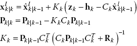
At time k, the estimate of the state vector is denoted by ![]() and its covariance matrix is represented by Pk. Inasmuch as Pk is a positive definite matrix, its Cholesky decomposition is given by
and its covariance matrix is represented by Pk. Inasmuch as Pk is a positive definite matrix, its Cholesky decomposition is given by ![]() , where Sk is a positive lower triangular matrix. The n + 1 sigma points are selected as follows [24]:
, where Sk is a positive lower triangular matrix. The n + 1 sigma points are selected as follows [24]:
- Choose the equal weights as
 .
. - Construct the scale vectors as

- Arrange the sigma points in an
 matrix;
  , where
  represents the Kronecker product.
After the sigma points are chosen, they are propagated and updated according to the pseudo code in Table 18.1.
18.2.4 Results and Discussion
Numerical simulations performed in this subsection are meant to verify the performance of MUKF in the problem of gyro‐less COAD. As a demonstration of the capabilities of MUKF, a small LEO satellite is taken in its normal mode of operation. The states of the COAD problem are grouped in a vector ![]() The measurement pack consists of TAM and Sun sensors the noise of which are modelled as zero mean Gaussian white standard deviations of 50 nT and 1.8°, respectively. The geomagnetic field is also modelled using the 13th order IGRF 11 [21]. The estimation results are considered for seven orbital periods. Tables 18.2 and 18.3 show the initial conditions as well as the system data required for the simulation.
The measurement pack consists of TAM and Sun sensors the noise of which are modelled as zero mean Gaussian white standard deviations of 50 nT and 1.8°, respectively. The geomagnetic field is also modelled using the 13th order IGRF 11 [21]. The estimation results are considered for seven orbital periods. Tables 18.2 and 18.3 show the initial conditions as well as the system data required for the simulation.
Table 18.2 Initial simulation conditions for COAD.
| State | True values | Estimation values |
| ωBI (rad/s) | [0 −0.0011 0]T | [1e − 3 −0.002 1e − 3]T |
| {q} | [−0.0739 −0.7032 −0.5495 −0.4450]T | [0.5359 −0.4794 0.3806 0.5814]T |
| a (km) | 7078.145 | 6778.145 |
| E | 0.07 | 0.1 |
| i (°) | 70 | 50 |
| Ω (°) | 57 | 45 |
| ω (°) | 0 | 17.18 |
| M (°) | 0 | 17.18 |
Table 18.3 System and simulation data for COAD.
| Mass (kg) | 40 |
|
|
diag([1.2 1 1.1]) |
| Qω |
|
| Qα |
|
| Sampling interval (s) | 10 |
Applying UKF to the prescribed COAD problem shows that mean average run time over ten Monte Carlo simulations is about 1740 s, while it only takes only 900 s for the MUKF to achieve a similar accuracy level. This comparison indicates that MUKF has made a 48% reduction in run time, and is therefore definitely more efficient and advantageous for online applications. The problem was analyzed on a PC computer with 4 Gb RAM and a CPU of 2.53 GHz. In the next sections, additional details of the results and their analyses are presented.
Estimation Results and Analysis
Figures 18.2–18.4 show true and estimated states in the coupled roto‐translational dynamics for up to seven orbital periods for a sample simulation. As shown in these figures, initial fluctuations have diminished over less than two orbital periods and the estimation of the whole system states that include the orbital parameters have converged to their true values after two orbital periods.

Figure 18.2 Time history of true and estimated angular velocity vector.
![4 Graphs of t [revolution] vs. q1, q2, q3, and q4 (top to bottom) illustrating time history of true and estimated quaternion parameters depicted by solid (true) and dashed (MUKF) lines.](http://images-20200215.ebookreading.net/13/1/1/9781118928684/9781118928684__advanced-uav-aerodynamics__9781118928684__images__c18f003.gif)
Figure 18.3 Time history of true and estimated quaternion parameters.
![6 Graphs of t [revolution] vs. a [km], i [deg], ω [deg], e, Ω [deg], and M [deg] illustrating time history of true and estimated orbital elements depicted by solid (true) and dashed (MUKF) lines.](http://images-20200215.ebookreading.net/13/1/1/9781118928684/9781118928684__advanced-uav-aerodynamics__9781118928684__images__c18f004.gif)
Figure 18.4 Time history of true and estimated orbital elements.
To study the performance of the MUKF algorithm, a Monte Carlo simulation is also performed on the noise characteristics of the measurement package. Root mean‐square error (RMSE) values of the error magnitudes for attitude, angular velocity magnitude and the orbital elements over ten Monte Carlo simulations are shown in Figures 18.5 and 18.6. These figures show that the large initial errors for the state vector have gradually decreased to zero as the observation data is fed in to the algorithm, indicating good robustness of the MUKF. Magnification of the results illustrates that the AD achieves accuracy levels of better than 0.3° in attitude estimation and better than 0.003°/s in body angular rates. In addition, the OD navigation accuracy in terms of the satellite position and velocity are about 3.85 km and 0.5 m/s respectively along each axis, which is very good considering the use of MEMS sensors in the measurement package.

Figure 18.5 RMSE of attitude and norm of angular velocity.
![6 Graphs of t [revolution] vs. RMSE (a) [km], RMSE (i) [deg], RMSE (ω) [deg], RMSE (e), RMSE (Ω) [deg], and RMSE (M) [deg] displaying descending plots.](http://images-20200215.ebookreading.net/13/1/1/9781118928684/9781118928684__advanced-uav-aerodynamics__9781118928684__images__c18f006.gif)
Figure 18.6 RMSE of orbital elements.
A summary of this MEMS‐based COAD research in comparison with the recent Gyro‐less work is presented in Table 18.4. As this table shows, despite inclusion of disturbing forces and moments, appropriate selection of a measurement package (sensors) combined with proper implementation of the MUKF filter has improved the attitude and position estimation accuracy without the need for any true/pseudo gyro measurement.
Table 18.4 A comprehensive summary of COAD studies in terms of estimation accuracy [20].
| Ref | Sensor(s) | Orbit | Filter | Accuracy | |||
|
Position (km) |
Velocity (m/s) |
Attitude (°) |
Att. rate (°/s) | ||||
| [16] | Gyro, TAM | Non‐Keplerian. | EKF | 30 | 30 | 0.7–1.4 | — |
| [17] | Gyro, TAM | Keplerian. | EKF | — | |||
| [18] | Gyro, TAM | Keplerian. | UKF | 5 | 20 | 0.2 | — |
| [19] | TAM, TAM rate | Non‐Keplerian. | EKF | 8 | 5 | 5 | 0.03 |
| Current work | TAM, Sun sensor | Non‐Keplerian. | MUKF | 3.85 | 0.5 | 0.3 | 0.003 |
Covariance Analysis and Observability
As the state‐estimation problem reconstructs the system states using available observations, system observability demonstrates a uniqueness recovery of the system states from the observed data. In this sense, observability is a prerequisite for successful estimation. A system is theoretically observable if the so‐called observability matrix (OM) is of full rank [25]. By investigating the roto‐translation dynamic system with the observation model, one can guarantee local observability via assessment of the OM rank. The OM rank over the whole sampling time equals 12, indicating full observability of the COAD problem.
The standard deviations of the estimated state vector elements are also a suitable measure to assess the system observability [1]. In other words, if the square roots of the diagonal elements of ![]() are small in a problem‐dependent sense, the system is observable in practice. Since the covariance of the estimated vector is equal to the inverse of the observability Gramian of the linearized system, small values of these quantities imply that the state error covariance matrix is nonsingular, which in turn implies system observability.
are small in a problem‐dependent sense, the system is observable in practice. Since the covariance of the estimated vector is equal to the inverse of the observability Gramian of the linearized system, small values of these quantities imply that the state error covariance matrix is nonsingular, which in turn implies system observability.
Figures 18.7–18.9 illustrate a decreasing trend of the standard deviations, as described above, to acceptable small levels, reaffirming the observability of the proposed system. The time histories of the state standard deviations are plotted for three orbital periods.

Figure 18.7 Square root of the diagonal elements of matrix P appropriated to the angular velocity components.

Figure 18.8 Square root of the diagonal elements of matrix P appropriated to the quaternion parameters.

Figure 18.9 Square root of the diagonal elements of matrix P appropriated to the orbital elements.
In this regard, it is important to note that in contrast with previous research [19], the proposed COAD problem has no need to include the time rate of the magnetic field as part of the measurement system to achieve complete observability; this is an additional advantage of the MUKF sensor package.
Sensitivity Analysis
The effect of various system and sensor parameters on the observability and estimation accuracy is analysed in this subsection. It is worth mentioning that the filter tuning is of significance in estimation accuracy, which means that good filter tuning can provide a more precise state estimation in a wide range of acceptable system and mission scenarios. It is also notable that to calculate the attitude estimation error, the quaternion error can be calculated as:
Since the fourth element of the quaternion is the scalar part related to the rotation angle, its estimation error can be computed as follows:
- Semi‐major axis effect: The effect of the orbital semi‐major axis on the absolute error of the estimated process is shown in Table 18.5, indicating that increasing the orbital altitude slightly reduces the estimation accuracy. The key reason for this effect is the altitude dependency of the Earth’s magnetic field, which reveals itself via the magnetometers and the IGRF model. As the geomagnetic field weakens with altitude, the precision of the state estimation decreases. Moreover, the attitudinal and orbital parameters are correlated. Attitude and orbital parameters are coupled through the perturbation forces, so a change in the orbital elements affects the attitudinal parameters. However, based on these observations, it is seen that even for severe cases, the estimation results are of good accuracy. Thus one could expect to use the tested algorithm for autonomous navigation and control in a wide range of small satellites in LEO missions.
- Orbit inclination effect: Orbit inclination is the most significant orbital parameter affecting observability. It is shown that increasing the orbit inclination improves the accuracy of state estimation. As the satellites moving in high‐inclined orbits pass over more asymmetrical regions of the Earth geomagnetic field, the observability is strengthened; thus, better estimation results are achieved. Expectedly, as Table 18.6 indicates, the semi‐major axis is the most affected parameter in this sensitivity.
- Measurement accuracy effect: It is intuitively obvious that more expensive accurate sensors improve state estimation accuracy. This fact is verified in Table 18.7. However, as shown in this table, good nonlinear filters such as the proposed MUKF can compensate for less accurate MEMS‐type sensors to provide an acceptable navigation subsystem.
- Initial angular velocity effect: Satellites can experience different angular velocities due to perturbations. The effect of initial angular velocity on the precision of the estimation results is presented in Table 18.8. As anticipated, MUKF has low sensitivity with respect to angular velocity forcing. This also shows that MUKF results can be reliable even during manoeuvring phases.
- Sampling rate effect: Data‐sampling rate directly influences the estimation accuracy. Table 18.9 clearly shows that increasing the sample rate prevents covariance growth, so a more precise estimation is achieved.
- Eclipse effect: It is obviously impossible to get any reliable measurements from the Sun sensor during eclipses. The effect of solar eclipses on the state estimation of roto‐translational dynamics is illustrated in Figures 18.10 and 18.11 over the first three orbital periods. The vertical dashed bars indicate the occurrence of eclipses. From these figures, the resulting accuracy is degraded in the first orbital period, but soon after, with little elapsed time and data processing, the MUKF has taken over and the state estimation process has recovered. Therefore, the proposed dynamics and the measurement systems are appropriate even during eclipses or even if the Sun sensor fails.
- Noise correlation effect: Correlation between the process and measurement noise seldom occurs in practice but is likely. To investigate the effect of noise correlation on the COAD performance, MUKF is improved using an idea inspired by the work of Xu et al. [26]. Figures 18.12–18.14 demonstrate the acceptable quality of estimation in this case as well.
- Moment of inertia effect: The moment of inertia (MOI) matrix is the most important parameter that affects the rotational dynamics of an orbiting satellite. In the current simulation, MOI has been so far considered as diag([1.2 1 1.1]), but in order to investigate its effect on COAD performance, it is changed to:

The time history of the estimation error is shown in Figures 18.15–18.17. These figures clearly show that not only has the estimation error not increased but also, because of more regular changes of angular velocity, the convergence time is improved too.
Table 18.5 Effect of the initial semi‐major axis on the estimation accuracy [20].
| h a [km] | Attitude error [°] | ‖Δa‖[km] | ‖Δe‖ | ‖Δi‖[°] | ‖ΔΩ‖[°] | ‖Δω‖[°] | ‖ΔM‖[°] |
| 600 | 0.2 | 0.3 | 1e − 4 | 0.08 | 0.09 | 0.1 | 0.08 |
| 700 | 0.3 | 0.4 | 1e − 4 | 0.1 | 0.1 | 0.2 | 0.1 |
| 800 | 0.45 | 0.7 | 1e − 4 | 0.2 | 0.17 | 0.22 | 0.1 |
Table 18.6 Effect of the orbit inclination on the estimation accuracy [20].
| i[°] | Attitude error [°] | ‖Δa‖[km] | ‖Δe‖ | ‖Δi‖[°] | ‖ΔΩ‖[°] | ‖Δω‖[°] | ‖ΔM‖[°] |
| 50 | 0.35 | 0.6 | 3e − 4 | 0.13 | 0.12 | 0.22 | 0.12 |
| 70 | 0.3 | 0.4 | 1e − 4 | 0.1 | 0.1 | 0.2 | 0.1 |
Table 18.7 Effect of the TAM standard deviation on the estimation accuracy [20].
| σ TAM [nT] | Attitude error [°] | ‖Δa‖[km] | ‖Δe‖ | ‖Δi‖[°] | ‖ΔΩ‖[°] | ‖Δω‖[°] | ‖ΔM‖[°] |
| 30 | 0.2 | 0.3 | 1e − 4 | 0.04 | 0.07 | 0.15 | 0.03 |
| 50 | 0.3 | 0.4 | 1e − 4 | 0.1 | 0.1 | 0.2 | 0.1 |
| 70 | 0.4 | 0.7 | 1e − 2 | 0.2 | 0.5 | 0.34 | 0.12 |
Table 18.8 Effect of the initial angular velocity on estimation accuracy [20].
| ω 0[rad/s] | Attitude error [°] | ‖Δa‖[km] | ‖Δe‖ | ‖Δi‖[°] | ‖ΔΩ‖[°] | ‖Δω‖[°] | ‖ΔM‖[°] |
|
|
0.35 | 0.5 | 2e − 4 | 0.2 | 0.18 | 0.3 | 0.12 |
| ω 0 | 0.3 | 0.4 | 1e − 4 | 0.1 | 0.1 | 0.2 | 0.1 |
Table 18.9 Effect of sample rate on the estimation accuracy [20].
| Data sampling rate [Hz] | Attitude error [°] | ‖Δa‖[km] | ‖Δe‖ | ‖Δi‖[°] | ‖ΔΩ‖[°] | ‖Δω‖[°] | ‖ΔM‖[°] |
| 1 | 0.2 | 0.3 | 5e − 5 | 0.02 | 0.02 | 0.015 | 5e − 3 |
| 0.1 | 0.3 | 0.4 | 1e − 4 | 0.1 | 0.1 | 0.2 | 0.1 |
Figure 18.10 RMSE of orbital elements considering eclipse durations.
Figure 18.11 RMSE of attitude and angular velocity considering eclipse durations.

Figure 18.12 Time history of estimation error in quaternion parameters

Figure 18.13 Time history of estimation error in angular velocity components.

Figure 18.14 Time history of estimation error in orbital elements.

Figure 18.15 Time history of estimation error in angular velocity components.

Figure 18.16 Time history of estimation error in quaternion parameters.

Figure 18.17 Time history of estimation error in orbital elements.
18.3 Concurrent Attitude and System Identification
Accurate knowledge of SC attitude, attitude rate and system parameters is vital for the performance of space tasks such as remote sensing, imaging, pointing, and data transmission. It is important to note that the SC attitude and attitude rate are required to implement closed‐loop attitude control for keeping SCs on station or manoeuvring them. But for many space missions there is a direct relationship between accurate identification of the SC system parameters and the desired level of mission success and/or achievements. In this respect, the MOI tensor is one of the key system characteristics, and significantly affects the satellite rotational dynamics and the control subsystem design. In short, not only the SC states, but also its system parameters and the error parameters involved in the measurement package, need to be accurately identified to achieve accuracy and reliable performance. As operational and environmental conditions of orbiting SCs may vary considerably from those assumed in the design and simulation phases, online estimation of dynamics and the measurement system’s parameters are of the utmost importance. This section is devoted to concurrent estimation of satellite’s attitude, MOI, and the sensor error parameters.
18.3.1 Dynamic System with Sensor Parameter Estimation
A Bayesian framework is used to simultaneously estimate the SC states and parameters. To this end, the nonlinear attitude dynamics of the satellite (Table 18.3) are described by Eq. (18.3). The model assumes that the aerodynamic drag and gravity gradient forces are the most effective forces that produce torques for the selected LEO satellite (described by Eqs (18.4) and (18.5)). The effect of the other perturbing torques can be modelled as process noise.
Again, a centralized data fusion of TAM and Sun sensors provides the measurement data. However, in this case the TAM measurements are assumed to be contaminated with various sources of error – such as the scale factor, misalignment, bias, and random white noise [27] – the accurate online estimation of which is part of the problem:
in which
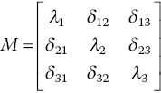
whose diagonal elements represent the scale factors, with the misalignment parameters in the off‐diagonal elements. b represents the bias vector and vB is the measurement white noise with a predefined covariance. Finally, E represents a 3 × 3 unit matrix.
The Sun sensor is again as modelled as in Eq. (18.16). The Sun sensor errors are usually negligible in comparison with those of the TAMs, which is a logical assumption. Further, it is assumed that the SC navigational data (position and velocity) is available via an orbital determination subsystem. It needs to be mentioned that are parameters needing estimation are modelled as random constants.
18.3.2 Persistence of Excitation
Complete observability requirement of the complex problem introduced in this section demands satellite manoeuvring for identification purposes. In other words, in order to achieve simultaneous estimation of the SC states, MOI and the TAM parameters, persistent excitation must be guaranteed. As one of the reference manoeuvre trajectories that satisfies the required condition of persistent excitation, the following rate trajectory is used [28]:

where ![]() , and
, and ![]() . Figure 18.18 shows the proposed reference manoeuvre trajectory. The overall manoeuvre time is taken to be 15 min.
. Figure 18.18 shows the proposed reference manoeuvre trajectory. The overall manoeuvre time is taken to be 15 min.
Figure 18.18 Body angular rate command trajectory.
18.3.3 Marginal Minimum Sigma Point Kalman Filter
As pointed out in Section 18.2, the nonlinear problem of SC AD has been extensively investigated over the past couple of decades using ideas and algorithms the details of which are beyond the scope of this chapter. Although EKF has been widely studied and utilized for AD in many previous papers, sample‐based algorithms such as MUKF, discussed in Subsection 18.2.3, are emerging rapidly, and are more suitable for online applications in nonlinear systems.
Although MUKF is by itself an efficient algorithm for practical applications, marginalization of partially linear systems, such as that of MSC, can effectively enhance its efficiency via reduction of its computational complexity. The basic idea behind marginalization is to partition the state vector into two parts: a linear part xl and a nonlinear part xn. In the framework of Bayes’ rule, the linear state variables can then be marginalized out and estimated using the basic optimal linear Kalman filter (KF). The nonlinear state variables are to be estimated using MUKF. In this way, marginal MUKF (MMUKF) only needs one set of sigma points that adequately describes the statistical properties of the nonlinear part of the state vector. This technique is also referred to as Rao–Blackwellization. While the basic idea of marginal filters and Rao‐Blackwellization is also applied for PF, its application to the UKF is new and useful [29].
In our case study, the dimension of the state vector is high (n = 25), while at the same time, only the kinematics and dynamics of the attitude system are nonlinear. Accordingly, MMUKF can be effectively utilized in this case. In this regard, TAM error parameters are estimated using the basic KF, while the MOI that appears nonlinearly in Euler equation of motion can be estimated via MUKF. Therefore, in conclusion, the MOI accompanied by the quaternion parameters and the body angular velocities are considered in the nonlinear part of the states, and are to be estimated using the MMUKF algorithm described in Table 18.10.
To introduce MMUKF, the dynamic and measurement systems are rewritten in discrete time form as:
where

x n is the n1‐dimensional nonlinear part of the state vector, xl is n2‐dimensional linear part of state vector (n1 + n2 = n) and zk is the m‐dimensional observation vector. In addition, f, h, Al, and C are some nonlinear functions. The process and the measurement noise vectors are wk and vk, respectively. Again, the noise vectors wk and vk are taken as zero‐mean Gaussian (white) with co‐variances given by Q k and Rk, respectively.
Table 18.10 The marginal modified unscented Kalman filter algorithm.
|


18.3.4 Results and Discussions
This subsection is devoted to the simulation results, which includes estimation of the system states, system parameters (MOI) and the parameters related to the measurement system. Given the discussions of Section 18.3.3, the nonlinear part of the state vector is ![]() and the linear part contains the measuring‐system‐related parameters
and the linear part contains the measuring‐system‐related parameters ![]() , where
, where ![]() ,
, ![]() ,
, ![]() and
and ![]() .
.
The control torque required to implement the commanded manoeuvre is computed using a fuzzy self‐tuning PID controller [25]. Figure 18.19 depicts the time history of the input control torque components.

Figure 18.19 Time history of control torque components.
It needs to be mentioned that TAM and Sun sensor random noises are modelled as zero mean Gaussian white with standard deviations of 50 nT and 1.8° respectively. The geomagnetic field is modelled using the 13th order IGRF 11 [21]. Initial conditions for the simulation and orbit simulation are presented in Tables 18.11 and 18.12, respectively.
Table 18.11 Initial simulation conditions.
| State | Initial true values | Initial estimated values |
| Angular velocity (rad/s) | [0 −0.0011 0] | [1e − 3 −0.002 1e − 3] |
| Quaternion parameters | [−0.0739 −0.7032 −0.5495 −0.4450] | [0.4063 0.7592 −0.3573 −0.3617] |
| MOI (kg.m2) |
[200 50 −30 50 240 10 −30 10 100] |
[160 20 −20 20 160 −20 −20 −20 160] |
| Scale factors (ppm) | [5 −1 −2]e + 4 | [0 0 0] |
| Misalignments (arcs) |
[648 1296 972 648 −648 1296] |
[0 0 0 0 0 0] |
| Bias (nT) | [1500 1000 500] | [0 0 0] |
Table 18.12 Initial orbit conditions.
| Element | Value | Element | Value |
| Semi‐major axis (km) | 7078.145 | Eccentricity | 0.07 |
| Inclination (°) | 70 | Longitude of ascending node (°) | 57 |
| Argument of perigee (°) | 0 | Mean anomaly (°) | 0 |
The measurement sampling interval is taken as 0.2 s. ![]() is considered as a diagonal matrix, with elements equal to
is considered as a diagonal matrix, with elements equal to ![]() for body angular velocities and zero for the other nonlinear states. Since all the parameters needing estimation are modelled as random constants,
for body angular velocities and zero for the other nonlinear states. Since all the parameters needing estimation are modelled as random constants, ![]() is a 12 × 12 zero matrix as well.
is a 12 × 12 zero matrix as well.
Application of the three algorithms UKF, MUKF, and MMUKF to the current problem shows that the mean average run time of the MMUKF over ten simulations takes only about 1615 s, as opposed to 3588 s for the MUKF and 4957 s for the standard UKF. This comparison indicates that the MMUKF has caused a 68% reduction in run time relative to the standard UKF, and 55% relative to MUKF. Therefore, MMUKF is definitely more efficient for online applications. It also needs to be mentioned that the current problem is implemented and solved on a PC computer with 4G RAM and a CPU of 2.53 GHz.
To further demonstrate MMUKF efficiency, the results of its Monte Carlo simulations are now presented. Figures 18.20–18.25 show state estimation errors (solid lines) along with ±3σ error bounds (dashed lines) taken from the covariance matrix at every time step. This convergence pattern verifies the good performance of the algorithm and indicates that each variable has a different convergence time constant. Figures 18.20 and 18.21 show that the attitude and body angular velocity estimation errors converge within their respective 3σ value after only 40 s, indicative of near‐optimal performance of the MMUKF algorithm. Similarly, Figures 18.22–18.24 show convergence to 3σ bounds in 60 sec for the MOI estimation, 30 sec for the scale factors and 20 sec for the misalignment parameters. In contrast to fast convergence of the states and system parameters, it takes about 300 sec to have a converged bias estimation error as denoted in Figure 18.25. Table 18.13 summarizes the RMSE of the state vector.

Figure 18.20 Estimation error of quaternion parameters in MMUKF with ±3σ error bound.

Figure 18.21 Estimation error of body angular velocity in MMUKF with ±3σ error bound.

Figure 18.22 Estimation error of moments of inertia in MMUKF with ±3σ error bound.

Figure 18.23 Estimation error of scale factors in MMUKF with ±3σ error bound.

Figure 18.24 Estimation error of misalignments in MMUKF with ±3σ error bound.
Figure 18.25 Estimation error of biases in MMUKF with ±3σ error bound.
Table 18.13 RMSE of state vector.
Source: Kiani et al. (2014) [27].
| State | Root Mean Square Error | State | Root Mean Square Error |
| Angular velocity (rad/s) | 4e − 3 | Scale factors (ppm) | [250 200 2000] |
| Rotation angle (deg) | 1.4 | Misalignments (arcs) | [100 200 800 270 200 200] |
| MOI (kg.m2) |
[1.6 0.5 0.01 0.5 1.9 0.02 0.01 0.02 0.83] |
Bias (nT) | [1 25 4] |
18.4 Summary and Conclusions
Two important topics of spacecraft navigation related to concurrent orbit and attitude determination as well as concurrent system and parameter identification plus sensor calibration are described.
The first part described the feasibility of concurrent gyro‐less orbit and attitude estimation for small LEO satellites using a centralized data fusion scheme with a TAM and a Sun sensor. The MUKF was implemented as a robust tool that results in acceptable accurate estimations; its major advantage is the use of a minimum number of sigma points, within the family of sigma point Kalman filters, causing a 48% run time reduction in comparison with standard UKF while preserving the same level of accuracy.
The stability and performance of MUKF were demonstrated via Monte Carlo simulations for a typical LEO satellite. A comprehensive sensitivity analysis over different effective parameters, such as orbital elements, TAM standard deviations and eclipse durations, was performed as part of the numerical simulation in Subsection 18.2.4. The results are promising and indicative of improved and enhanced state‐of‐the‐art capabilities in the COAD estimation problem. The results also indicate that the achieved levels of accuracy satisfy the navigation and control subsystem qualification requirements of small satellites.
In the second part, the complex high‐dimensional problem of concurrent attitude determination (AD), parameter identification (PI) and measurement sensor calibration (MSC) was developed and investigated. Accordingly, the SC attitude, attitude rates, moments of inertia tensor (MOI) plus the measuring system parameters, including scale factors, misalignments and biases of the TAMs, were recursively and simultaneously estimated based on the central fusion of the TAM and Sun sensor data. As the pertinent governing system model of the considered problem is a mixture of linear and nonlinear equations, an advanced marginal modified unscented Kalman filter – the marginal modified UKF (MMUKF) – consisting of a Kalman filter (KF) and MUKF was introduced. MMUKF was implemented as a robust tool which gives acceptably accurate estimations for the complex problem posed. MMUKF uses only 14 sigma points to estimate a full 25‐dimensional state vector in the case study considered, while standard UKF needs 52 sigma points and MUKF requires 26 sigma points for the same problem. Application of MMUKF has reduced the run time by about 68% as compared with the standard UKF, while preserving the same accuracy level. Stability and performance of the mixed problem of AD, PI and MSC using the proposed MMUKF algorithm were demonstrated via Monte Carlo analysis for a LEO satellite. The results are promising and indicative of a good state‐of‐the‐art capability for simultaneous AD, PI and MSC state/system estimation using a low‐cost MEMS TAM plus a Sun sensor measurement package.
References
- 1 L. Psiaki M., ‘Autonomous LEO orbit determination from magnetometer and sun sensor data’, AIAA Paper 98‐4308, 1998, pp. 1–12.
- 2 Y.T. Chiang, L.S. Wang, F.R. Chang, and H.M. Peng, ‘Constrained filtering method for attitude determination using GPS and gyro’, IEEE Proceedings‐Radar Sonar and Navigation, 149 (5), 2002, pp. 258–264.
- 3 Ma Zi, A. Ng, ‘Spacecraft attitude determination by adaptive Kalman filtering’, AIAA Modelling and Simulation Techniques Conference and Exhibit, California, 2002. AIAA Paper 2002‐5042.
- 4 J.L. Crassidis and F.L. Markley, ‘Unscented filtering for spacecraft attitude estimation’, Journal of Guidance, Control and Dynamics, 26 (4), 2003, pp. 536–542.
- 5 D. Choukroun, I.Y. Bar‐Itzhack, and Y. Oshman, ‘Optimal‐REQUEST algorithm for attitude determination’, Journal of Guidance, Control and Dynamics, 27 (3), 2004, pp. 418–425.
- 6 A. Carmi and Y. Oshman, ‘Robust spacecraft angular rate estimation from vector observations Using interlaced particle filtering’, Journal of Guidance, Control and Dynamics, 30 (6), 2007, pp. 1729–1741
- 7 T. Xu, G. Gu, and X. Shen, ‘A maneuvered GEO satellite orbit determination using robustly Adaptive Kalman filter’, Proceeding of International Conference on Intelligent System Design and Engineering Application, Vol. 1, 2010, pp. 55–59.
- 8 B. Ristic, S. Arulampalam, N. Gordon, Beyond the Kalman Filter, Particle Filters for Tracking Applications, Artech House, 2004.
- 9 D.M. Shuster, ‘A survey of attitude representations’, Journal of the Astronautical Sciences, 41 (3), 1993, pp. 439–517.
- 10 P.H. Zipfel, Modeling and Simulation of Aerospace Vehicle Dynamics. AIAA, New York, 2000, pp. 122–125 and 181–185.
- 11 M.J. Sidi, Spacecraft Dynamics and Control, A Practical Engineering Approach. 1st edn, Cambridge University Press, New York, 1997, pp. 30–33 and 95–96.
- 12 G.R. Hintz, ‘Survey of orbit element sets’, Journal of Guidance, Control, and Dynamics, 31 (3), 2008, pp. 785–790.
- 13 H.D. Curtis, Orbital Mechanics for Engineering Students, 2nd edn, Elsevier, 2010, pp. 208–212.
- 14 D.A. Vallado, W.D. McClain, Fundamentals of Astrodynamics and Applications, 4th edn, Microcosm Press and Springer, (2013), pp. 279–280, 303, 565, and 637.
- 15 J. Bae and K. Youan, ‘Attitude estimation for satellite fault tolerant system using federated unscented Kalman filter’, International Journal of Aeronautical and Space Sciences, 11 (2), 2010, pp. 80–86.
- 16 J.K. Deutschmann, I.Y. Bar‐Itzhack, ‘Comprehensive evaluation of attitude and orbit estimation using actual earth magnetic field data’, Journal of Guidance, Control, and Dynamics, 24 (3), 2001, pp. 616–635.
- 17 W.Jianqi, C. Xibin, and S. Zhaowei, ‘Attitude and orbit determination for small satellite using magnetometer measurement’, Aircraft Engineering and Aerospace Technology, 75 (3), 2003, pp. 241–246.
- 18 Y. Xing, X. Cao, S. Zhang, ‘Modified UKF for integrated orbit and attitude determination based on gyro and magnetometer’, 2nd International Symposium on Systems and Control in Aerospace and Astronautics, 2008, pp. 1–4.
- 19 M. Abdelrahman, S.‐Y. Park, ‘Simultaneous spacecraft attitude and orbit estimation using magnetic field vector measurements’, Aerospace Science and Technology, 15 (8), 2011, pp. 653–669.
- 20 M. Kiani, Seid H. Pourtakdoust, ‘Concurrent orbit and attitude estimation of LEO satellites using minimum sigma points UKF’, Proceedings of the Institute of Mechanical Engineers Part G: Journal of Aerospace Engineering, 228 (6), 2013, pp. 810–819.
- 21 C.C. Finlay, S. Maus, C.D. Beggan et. al., ‘International Geomagnetic Reference field: the eleven generation’, Geophysical Journal International, 183, 2010, pp. 1216–1230.
- 22 S.J. Julier and J.K. Uhlmann, ‘A new extension of the Kalman filter to nonlinear systems’, in Proceedings Of Aero Sense: The 11th Int. Symposium on Aerospace/Defence Sensing, Simulation and Controls, Orlando, 1997, pp. 54–65.
- 23 S.J. Julier, ‘The spherical simplex unscented transformation’, in Proceedings of the American Control Conference, Denver, Colorado, 2003, pp. 2430–2434.
- 24 W.‐.Ch. Li, P. Wei, and X.‐C. Xiao, ‘Novel simplex unscented transform and filter’, Journal of Electronic and Technology of China, 6 (1), 2008, pp. 61–65
- 25 L.X. Wang, A Course in Fuzzy systems and Control, Prentice Hall, 2002, pp. 257–258.
- 26 J. Xu, G.M. Dimirovski, Y. Jing, and C. Shen, ‘UKF design and stability for nonlinear stochastic systems with correlated noises’, Proceedings of the 46th IEEE Conference on Decision and Control, New Orleans, LA, USA, 12–14 December 2007.
- 27 M. Kiani, Seid H. Pourtakdoust, ‘Spacecraft attitude and system identification via marginal reduced UKF utilizing the Sun and calibrated TAM sensors’, Scientia Iranica, 21 (4), 2014, pp. 1451–1460.
- 28 H. Myung, K. ‐L. Yong and H. Bang, ‘Hybrid estimation of spacecraft attitude dynamics and rate sensor alignment parameters’, International Conference on Control, Automation and Systems, 2007.
- 29 M. Briers, S.R. Maskell and R. Wright R., ‘A Rao‐Blackwellised unscented Kalman filter’, in Proceedings of 6th International Conference of Information Fusion, Queensland, Australia, 2003.