6
Chord‐dominated Ground‐effect Aerodynamics of Fixed‐wing UAVs
Qiulin Qu1 and Ramesh K. Agarwal2
1 Beijing University of Aeronautics and Astronautics, Beijing, China
2 Washington University in St. Louis, St. Louis, MO, USA
6.1 Introduction
The UAV is an acronym for ‘unmanned aerial vehicle’, an aircraft with no pilot on board. UAVs can be remote‐controlled (flown by a pilot at a ground control station) or can fly autonomously based on pre‐programmed flight plans or more complex dynamic automation systems. Currently, UAVs are widely used for military and civilian operations. UAVs can be classified into
- horizontal take‐off and landing fixed‐wing UAVs
- vertical take‐off and landing (VTOL) rotor UAVs.
During take‐off and landing on a runway or on an aircraft carrier deck, the aerodynamics and flow field of a fixed‐wing UAV will be influenced by the ground effect (GE). Ever since the early days of aviation, pilots have experienced the GE phenomenon while operating very close to the ground. Either during take‐off or landing, air vehicles experience improved efficiency near the ground in the form of increased lift.
When the aerodynamics are changed by GE during take‐off and landing, the pilot of a crewed aircraft can adjust its attitude in real time. However, it is difficult for the remotely operated UAV or the automatic control system of a UAV to do the same thing in real time. Thus, an understanding of their GE aerodynamics will benefit the development of automatic takeoff and landing systems for UAVs.
Nomenclature
In this chapter, the following nomenclature is used:
- A
- area of the channel between the lower surface of the airfoil and the ground
- CD
- drag coefficient
- CL
- lift coefficient
- Cp
- pressure coefficient
- c
- chord length of the airfoil
- DGE
- dynamic ground effect
- d
- width of local stream tube
- din
- width of the stream tube on the inlet boundary
- GE
- ground effect
- h
- ride height; the distance between the lowest point on the airfoil surface and the ground/the top of the platform
- j
- unit vector along y‐axis
- L
- the distance between the leading edge of airfoil and the side of platform
- MGE
- mutational ground effect
- Ma
- Mach number
- n
- unit vector normal to the airfoil surface
- p
- local static pressure
- p∞
- freestream pressure
- Re
- Reynolds number based on airfoil chord length
- S
- surface area of the airfoil
- SGE
- static ground effect
- T
- oscillation period of unsteady aerodynamic forces
- Vs
- sink velocity
- V∞
- freestream velocity
- W
- compression work done by the airfoil
- x, y
- Cartesian coordinates with the origin located at the leading edge of the airfoil
- y+
- dimensionless wall distance of the first mesh layer
- α
- angle‐of‐attack (AOA)
- β
- velocity vector angle; the angle between a velocity vector and the positive direction of the x‐axis
- γ
- flight path angle
- θ
- pitch angle
- Γ
- circulation around the airfoil
- ΔCL
- increment in lift coefficient
- (ΔCL)R
- dimensionless lift coefficient increment in the MGE
- Δt
- time step for unsteady simulation
- Δα
- increment in angle‐of‐attack (AOA)
- ρ
- air density
- τ
- shear stress on the airfoil surface
- Subscripts
- h
- ground effect with the ride height of h
- low
- lower surface of the airfoil
- up
- upper surface of the airfoil
- ∞
- unbounded flow
6.2 Categories of Ground Effect
Based on flow physics, the GE can be categorized into the attached‐flow GE of high‐aspect‐ratio wings for transport aircraft and the separated‐flow GE of delta wings for fighters. The former can be further classified into the chord‐dominated GE and the span‐dominated GE (Rozhdestvensky 2006). For a 2D airfoil at positive angle of attack (AOA), ground proximity generally causes a high‐pressure distribution on the lower surface of the airfoil leading to increase in lift, nose‐down pitching moment and the lift‐to‐drag ratio; this phenomenon is called the 2D chord‐dominated GE. For a 3D wing at positive AOA, ground proximity often pushes the wingtip vortices outward along the span leading to a decrease in downwash angle and induced drag; this phenomenon is called the 3D span‐dominated GE.
Depending on the application, the GE can be categorized into the static ground effect (SGE, in which the ride height does not change with time), the dynamic ground effect (DGE, in which the ride height changes continuously with time) and the mutational ground effect (MGE, in which the ride height changes suddenly with time) (Figure 6.1; see also Qu et al. 2015b). Wing‐in‐ground (WIG) craft use the SGE to improve the aerodynamic efficiency while cruising on the water surface (Qu et al. 2014); conventional aircraft undergo the DGE during taking‐off and landing (Qu et al. 2014b); fixed‐wing carrier aircraft undergo the MGE effect during taking‐off and landing on carrier decks (Coton 1998).

Figure 6.1 Category of GE based on application areas.
6.3 Chord‐dominated Static Ground Effect
For the 2D chord‐dominated GE, the aerodynamics and flow physics at low‐to‐moderate AOA have been extensively investigated. Hsiun and Chen (1996) studied the effect of camber and thickness on the aerodynamics of a 2D airfoil in the SGE by numerical simulation. They found that the aerodynamic forces on the airfoil were determined by the passage between the lower surface of the airfoil and the ground. Chun and Chang (2003) numerically simulated the flow fields around a Clark‐Y airfoil at α = 5.92° and a NACA4412 airfoil at α = 5° in the SGE using fixed and moving grounds. Their investigation indicated that there were very small differences in lift and pitching moment predictions between the results with fixed and moving grounds, but the drag in the fixed‐ground simulation was smaller than that in the moving‐ground simulation. Ahmed et al. (2007) reported experimental results for a NACA4412 airfoil in GE at α = 0–10°. They found that when the ride height was reduced, the drag increased, but the lift trend depended on the shape of the passage between the lower surface of the airfoil and the ground, which changed with the AOA. Zerihan and Zhang (2000) and Mahon and Zhang (2005) performed numerical simulations and wind tunnel experiments to study the negative GE of a Tyrrell‐02 airfoil, which is a highly cambered inverted airfoil. When the ride height decreased, the downward force first increased gradually to a peak value and then decreased dramatically.
The archival information about GE aerodynamics at high AOAs is very limited. Hiemcke (1997) has reported experimental results for a NACA5312 airfoil in GE at high AOA. It was found that the attached flow on the airfoil evolved into separated flow when the ride height was reduced at high AOA. However, Hiemcke has not described the physical reasons behind the occurrence of flow separation and the influence of flow separation on the aerodynamic forces. Ying et al. (2010) conducted numerical studies on the stall characteristics of a NACA0012 airfoil in GE. They found that the stall AOA decreased with the reduced ride height, but did not show the flow structure or explain the reasons behind what they observed.
Here, the aerodynamics and flow physics of a NACA4412 airfoil in the SGE for a wide range of AOA (Qu et al. 2015a) are discussed.
6.3.1 Physical Model
A NACA4412 airfoil with c = 1.0 m, Ma = 0.26 and Re = 6 × 10⁶ is investigated. A wide AOA range of α = −4–20° (with Δα = 2°) is considered in order to study both the attached and separated flow patterns in GE. For 2D chord‐dominated GE, several studies have concluded that the critical ride height (defined as the minimum height below which the aerodynamics is affected by the GE) is approximately h/c = 1.0 for low and moderate AOAs. Thus, relative ride heights of h/c = ∞, 1.0, 0.8, 0.6, 0.4, 0.2, 0.1 and 0.05 are considered. Values of h/c = 5.0 and 2.0 are additionally considered for cases of α = 4° and 8°.
Here the relative motion principle is adopted. The airfoil is fixed in space; the ground and the inflow from upstream move opposite to the flight velocity of the airfoil.
6.3.2 Lift Characteristics
For convenience in explaining the results, the following definitions and notations related to lift coefficient are introduced. The total lift coefficient of an airfoil is defined as follows:

The upper surface lift coefficient of an airfoil is defined as follows:

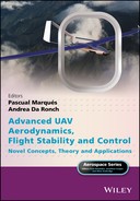
The lower surface lift coefficient of an airfoil is defined as follows:
The total lift is written as:
For the GE flow field with ride height h, the lift increments in total, upper surface and lower surface lifts due to GE are defined as follows:
The lift curves and lift increment curves of the NACA4412 airfoil at various ride heights are shown in Figure 6.2. The total lift curve in unbounded flow has an expected linear portion in the AOA range from −4–8°. However, the total lift curve in GE has a convex portion instead of a linear portion in this range. Therefore, there are two intersection points between the two lift curves: the lift curve in GE and the lift curve in unbounded flow. The smaller the ride height, the bigger are the curvatures of the convex portion of the airfoil and the AOAs corresponding to the intersection points. In the two regions outside the two intersection points, the lift decreases with the reduced ride height. In the region between the two intersection points, the lift increases with decreasing ride height; this is the region where traditional GE aerodynamics research has focused so far. All the cases in unbounded flow and the GE flow field for this airfoil have the same stall AOA of 16°. However, compared to the unbounded flow, in GE the maximum lift is smaller for h/c = 1.0–0.1 and is larger for h/c = 0.05. The stall characteristics become sharper for h = 0.1 and 0.05.


Figure 6.2 Lift curves and lift increment curves for the NACA4412 airfoil at various ride heights.
For all AOAs, the upper surface of the airfoil generates positive lift, which decreases with the reduced ride height. The larger the AOA, the greater is the decrease in the upper surface lift. For low, moderate and high AOA, the lower surface produces positive lift, which increases with the reduced ride height. For negative AOA, the lower surface produces negative lift, which decreases with the reduced ride height.
Previous investigations have determined that the critical ride height is approximately h/c = 1.0 for the 2D chord‐dominated GE at low and moderate AOAs. From Figure 6.2a, one can see that the critical ride height changes with AOA. For negative to moderate AOA, say −4° < α ≤ 8°, the critical ride height can be seen as approximately one chord; but for high AOA, say, 8° < α ≤ 20°, the critical ride height is larger than one chord. Furthermore, when h/c decreases from ∞ to 1.0, the total lift does not change appreciably for negative to moderate AOA, but the variations in both the upper and lower surface lifts are obvious.
The lift increment contours of the NACA4412 airfoil in the AOA–ride‐height plane are shown in Figure 6.3. Based on the sign of the total lift increment value, the AOA–ride‐height plane can be divided into three regions (Figure 6.3a):
- Region I of positive GE
- Region II of negative GE
- Region III of negative GE.

Figure 6.3 Lift increment contours of the NACA4412 airfoil in the AOA–ride‐height plane.
The lift characteristics and flow physics for the typical AOAs in the three regions are analyzed in detail.
6.3.3 Effect of Low‐to‐moderate AOA
Lift and Pressure Distribution
For the low‐to‐moderate AOA range, when the ride height decreases, the airfoil enters Region I from Region II (Figure 6.3a). In this AOA range, we analyze the two typical cases with α = 4° and 8°, where the passage between the lower surface of the airfoil and the ground forms a typical convergent channel, as shown in Figure 6.4.

Figure 6.4 Convergent passage between the lower surface of NACA4412 airfoil and the ground at α = 8°.
Figure 6.5 shows the variations in lift and lift increment with ride height for α = 4° and 8°. In the following analysis, the ride height of h/c = 10 represents the unbounded flow.

Figure 6.5 Variations in lift and lift increment with ride height.
In the unbounded flow, CL,up is much greater than CL,low. When the ride height decreases, CL,up decreases gradually and CL,low increases gradually. The smaller the ride height, the faster is the increase in CL,low. Therefore, CL,low becomes larger than CL,up at very small ride height.
At some value of AOA, there is a ride height that results in ΔCL = 0, which divides the lift increment curve into two regions: the lift reduction region (Region II) and the lift enhancement region (Region I). The higher the AOA, the smaller is the ride height that gives ΔCL = 0; it is h/c = 0.6 for α = 4° and h/c = 0.3 for α = 8°.
From h/c = ∞ to the ride height for which ΔCL = 0, ΔCL is less than 0 since │ΔCL,up│ > │ΔCL,low│. In this region, the trend of total lift is dominated by the upper surface. From the ride height at which ΔCL = 0 to h/c = 0.05, ΔCL is greater than 0 since │ΔCL,up│ < │ΔCL,low│, and it increases dramatically. In this region, the trend of total lift is dominated by the lower surface.
Figure 6.6 shows the pressure coefficient distribution on the NACA4412 airfoil at various ride heights. For the two AOAs considered, there is hardly any change in the trend of pressure distribution with ride height. When the ride height is reduced, Cp,up increases first quickly and then slowly, resulting in a decrease in CL,up; Cp,low increases first slowly and then quickly, resulting in an increase in CL,low.

Figure 6.6 Pressure coefficient distributions on the NACA 4412 airfoil at various ride heights.
From h/c = ∞ to h/c = 0.2, the suction peak decreases continually to a minimum. When the ride height decreases, the airfoil suction peak increases slightly, creating a larger adverse pressure gradient in the chord‐wise direction. This is because the stagnation point moves backwards.
Flow Physics
Figure 6.7 shows the streamlines around the NACA4412 airfoil in the unbounded flow field and in the GE flow field with h/c = 0.1. There are two special streamlines in the flow field around an airfoil. One terminates at the stagnation point on the airfoil and the other begins from the trailing edge of the airfoil. The two streamlines are collectively referred to as the ‘stagnation streamline’, which divides the upstream inflow into two branches: one goes over the airfoil and the other goes under the airfoil. In the unbounded flow field and in the GE flow field, the stagnation streamlines are labeled as F1 and G1 respectively.


Figure 6.7 Streamlines around the NACA4412 airfoil; F0–F2, unbounded flow, G0–G2, GE with h/c = 0.1.
The stagnation streamline extends upstream to the location x/c = −40. Another two streamlines located above and under the stagnation streamline at an equal distance of din = 0.1c from it are released from the location of x/c = −40. These are labeled as (F0, F2) and (G0, G2) for the unbounded flow field and the GE flow field respectively (Figure 6.7). Note that the streamline G2 is coincident with the ground for the GE flow field of h/c = 0.1.
For the AOA producing positive lift, the airfoil induces the surrounding streamlines to deflect upwards. In the unbounded flow field, the streamline deflection region is very large in the whole flow field. However, in the GE flow field, this region is much smaller and is only in the vicinity of the airfoil. The streamlines G0–G2 remain straight until they approach the leading edge of the airfoil.
Figure 6.8 shows the deflection of the stagnation streamline with ride height. When the ride height decreases, the position where the deflection begins moves towards the airfoil.
Figure 6.8 Deflection position of the stagnation streamline with ride height.
In order to explain the reduction in streamline defection in GE flow field, the mirror‐image model (Mook and Nuhait 1989) for positive GE is introduced. This is shown in Figure 6.9. The clockwise circulation around the airfoil is defined as –ΓI and the anticlockwise image circulation below the ground is defined as ΓI. In the upstream and downstream regions, the image circulation ΓI induces downwash and upwash flow respectively, which makes the streamlines approach the ground.
Figure 6.9 Mirror‐image model of positive GE.
In GE, the reduction in streamlines’ upward deflection produces two results: one of reducing the effective AOA and the other of blocking the airflow below the airfoil.
Figure 6.10 shows the velocity vector angle (defined as the angle between the velocity vector and the positive direction of the x‐axis.) distribution on the stagnation streamline at α = 8°. When the ride height is reduced, the velocity vector angle decreases, resulting in the reduction of effective AOA. The smaller the ride height, the smaller is the effective AOA.

Figure 6.10 Velocity vector angle distribution on the stagnation streamline at α = 8°.
In both the unbounded flow field and the GE flow field, the streamlines (F1 and F2) and (G1 and G2) respectively form a typical stream tube below the NACA4412 airfoil. Figure 6.11 shows the width of the stream tube along the flow direction. The tube width almost retains the same value from the inlet to x/c = −1, and then increases sharply to a maximum at x/c ≈ 0 (corresponding to the leading edge). After that, the width decreases quickly until x/c = 1 (corresponding to the trailing edge), and then decreases slowly to the inlet value at x/c = 2.
Figure 6.11 Width of the stream tube below the NACA4412 airfoil along the flow direction.
It is clear that the width of the stream tube below the airfoil in the GE flow field is much larger than that in the unbounded flow field. This is because the airflow is blocked in the convergent passage below the airfoil, so the velocity decreases and the pressure rises. The smaller the ride height, more airflow is blocked.
In GE, the effective AOA decreases, which would make Cp,up increase and Cp,low decrease. The airflow is blocked, which would make Cp,low increase. The combination of the two effects makes both Cp,up and Cp,low increase.
When the ride height decreases from h/c = ∞ to the ride height for which ΔCL = 0, the reduction in effective AOA dominates, thus │ΔCL,up│ > │ΔCL,low│ and the total lift decreases, resulting in negative GE. When the ride height decreases from the ride height for which ΔCL = 0 to h/c = 0.05, the airflow‐blocking effect dominates, thus │ΔCL,up│ < │ΔCL,low│ and the total lift increases, resulting in positive GE.
6.3.4 Effect of High AOA
Lift and Pressure Distribution
In the high‐AOA range located in Region II (Figure 6.3a), we analyze the two typical cases with α = 16° and 18°, for which the passage between the lower surface of the airfoil and the ground is still a typical convergent channel. Figure 6.12 shows the variation of lift increment with ride height. When the ride height is reduced, ΔCL,up decreases and ΔCL,low increases. │ΔCL,up│ > │ΔCL,low│ in the entire ride height region and therefore the total lift increment is negative, resulting in negative GE. Note that ΔCL,up decreases sharply from h/c = 0.1 to 0.05 for α =18°; this is because the separated flow suddenly extends to the leading edge of the airfoil (see Figure 6.18).

Figure 6.12 Variation of lift increment with ride height.
Figure 6.13 shows the pressure coefficient distribution on the NACA4412 airfoil at various ride heights. When the ride height is reduced, Cp,up increases quickly and Cp,low increases slowly.
Figure 6.13 Pressure coefficient distributions on the NACA 4412 airfoil at various ride heights.
In the unbounded flow, when AOA increases, Cp,low increases and Cp,up decreases. The maximum value of Cp,low is limited to 1, but the minimum value of Cp,up is unrestricted. Thus the change in Cp,up is larger than that in Cp,low.
In GE, when AOA increases, the pressure increment of the lower surface due to the airflow‐blocking effect decreases and the suction decrement of the upper surface due to the reduction of effective AOA increases. Thus the positive GE in Region I evolves into the negative GE in Region II.
There is an obvious pressure plateau region near the trailing edge of the upper surface of the airfoil indicating flow separation. When the ride height is reduced, the pressure plateau region extends towards the leading edge. For the case of α = 18° and h/c = 0.05, nearly the entire upper surface is occupied by the pressure plateau region, which results in a steep reduction in upper surface lift and the total lift due to sharp stall characteristics.
Flow Physics
Figure 6.14 shows the streamlines around the NACA4412 airfoil in the unbounded flow field and the GE flow field at h/c = 0.1. Figure 6.15 shows the width of the stream tube below the airfoil along the flow direction. The main characteristics of the streamline deflection and the stream tube width are similar to that for the low‐to‐moderate AOA cases. However, it is a qualitative analysis (based on less accurate quantitative information) due to separated flow at high AOA.
Figure 6.14 Streamlines around the NACA4412 airfoil; Fo–F2, unbounded flow, G0–G2, GE with h/c = 0.1.

Figure 6.15 Width of the stream tube below the NACA4412 airfoil along the flow direction.
For low‐to‐moderate AOA, the upper surface flow remains attached in both the unbounded flow field and the GE flow field, so the streamlines G0 and F0 are almost coincident above the airfoil (see Figure 6.7). For high AOA, however, the upper surface separated flow region in the GE flow field is greater than that in the unbounded flow field, so the streamline G0 is located above F0 in the vicinity of the airfoil.
Figure 6.16 shows the steady separated flow pattern on the upper surface of the NACA4412 airfoil. When the ride height is reduced, the separation point moves towards the leading edge (Figure 6.17) and the separation region is enlarged since the adverse pressure gradient along the chord direction increases.
Figure 6.16 Steady separated flow region on the upper surface of the NACA4412 airfoil.

Figure 6.17 Position of separation point as a function of ride height.
From Figure 6.17, it can be noted that the change in the location of the separation point at α = 18° is very sharp as the ride height changes from h/c = 0.1 to 0.05. At h/c = 0.05, the separation point is located close to the leading edge and the separated flow is periodic. Figure 6.18 shows the unsteady separated flow in one period of oscillation. In the separation region, vortices are constantly shed from the leading edge and then merge downstream. The entire upper surface is occupied by the separated flow, resulting in a pressure plateau region on the entire upper surface of the airfoil (Figure 6.13b).

Figure 6.18 Unsteady separated flow on the upper surface of NACA4412 airfoil at α = 18° and h/c = 0.05.
6.3.5 Effect of Negative AOA
Lift and Pressure Distribution
In the negative AOA range located in Region III (Figure 6.3a), we analyze the typical case of α = −4° where the passage between the lower surface of the airfoil and the ground is a typical convergent‐divergent channel like a 2D Venturi tube (as shown in Figure 6.19). Thus the airflow first accelerates to a maximum velocity at the throat section and then decelerates gradually, resulting in a greater suction peak at the throat section.

Figure 6.19 Convergent‐divergent passage between the lower surface of the NACA4412 airfoil and the ground at α = −4°.
Figure 6.20 shows the variations in lift and lift increment with ride height. When the ride height is reduced, CL,up initially does not change and then increases slightly (h/c ≤ 0.1), and CL,low decreases first gradually and then dramatically. Thus the trend in total lift is determined by the lower surface, so CL decreases with reduced ride height.
Figure 6.20 Variations in lift and lift increment with ride height at α = −4°.
Figure 6.21 shows the pressure coefficient distribution on the NACA4412 airfoil at various ride heights for α = −4°. It is interesting to note that the suction region on the lower surface is apparent due to the Venturi effect. When the ride height is reduced, Cp,up initially does not change and then decreases slightly, and thus the suction peak on the lower surface increases and the suction region is enlarged.

Figure 6.21 Pressure coefficient distributions on the NACA 4412 airfoil at various ride heights for α = −4°.
Flow Physics
Figure 6.22 shows the streamlines around the NACA4412 airfoil at α = −4°. The lift is negative in the entire ride height range (see Figure 6.20a), so the airfoil induces the surrounding streamlines to deflect downwards, the opposite of what was seen in the above cases producing positive lift at positive AOA. The reduction in streamlines’ downward deflection in GE increases the effective AOA.
Figure 6.22 Streamlines around the NACA4412 airfoil at α = −4°; F0–F2, unbounded flow, G0–G2, GE with h/c = 0.1.
The mirror‐image model of negative GE for α = −4° is shown in Figure 6.23. Since the case of α = −4° in the unbounded flow generates negative lift, the circulation around the airfoil is anticlockwise and is defined as ΓIII; the image circulation below the ground is clockwise and is defined as − ΓIII. In the upstream and downstream regions, the image circulation induces upwash and downwash flow respectively, which makes the streamlines approach the ground.

Figure 6.23 Mirror‐image model of negative GE.
Figure 6.24 shows the width of the stream tube below the airfoil along the flow direction at α = −4°. Because the airfoil generates negative lift, the stream tube becomes narrow in the vicinity of the airfoil. The tube width in GE is much smaller than in the unbounded flow due to the Venturi effect, so the velocity increases and the pressure decreases. The smaller the ride height, more apparent is the Venturi effect.

Figure 6.24 Width of the stream tube below the NACA4412 airfoil along the flow direction at α = −4°.
In GE at α = −4°, the effective AOA increases, which makes Cp,up decrease (here the upper surface is the pressure side), especially at small ride height, and Cp,low increase (here the lower surface is the suction side). The Venturi effect is also enhanced, which makes Cp,low decrease dramatically. Since the increment effect of effective AOA is much weaker than the Venturi effect, the trend of total lift is decided by the Venturi effect.
6.3.6 Conclusions on Chord‐dominated Static Ground Effect
The AOA–ride‐height plane can be divided into three regions based on the sign of the lift increment value: Region I of positive GE and Regions II and III of negative GE.
For low‐to‐moderate AOA, when the ride height decreases, the airfoil enters Region I from Region II, and the pressure on the lower surface of the airfoil increases due to the airflow‐blocking effect from the convergent passage between the lower surface and the ground and the pressure on the upper surface increases due to the reduction of effective AOA as a result of reduction in streamlines’ upward deflection. In Region II, the airflow‐blocking effect is weaker than the reduction effect in effective AOA resulting in a negative lift increment; in Region I, the airflow‐blocking effect is stronger than the reduction effect in effective AOA resulting in a positive lift increment.
For high AOA located in Region II, when the ride height is reduced, the separation point moves towards the leading edge of the airfoil and the separated flow region is enlarged since the adverse pressure gradient along the chord direction increases. The pressure increment on the upper surface due to the enlarged flow separation region is greater than the pressure increment on the lower surface due to the airflow‐blocking effect; therefore the lift increment is negative.
For negative AOA located in Region III, when the ride height is reduced, the suction on the lower surface increases due to the Venturi effect from the convergent‐divergent passage between the lower surface and the ground. The Venturi effect is stronger than the increment effect of effective AOA due to reduced downward deflection of streamlines; therefore the lift increment is negative.
6.4 Chord‐dominated Dynamic Ground Effect
During take‐off and landing, an aircraft respectively moves away or towards the ground and its ride height above the ground changes continuously with time, so the air flow around the aircraft is unsteady. In the past, the majority of investigators have treated the DGE as quasi‐steady, but recent studies (Matsuzaki et al. 2008, Molina and Zhang 2011) indicate that the unsteady flow can be considered as quasi‐steady only when the sinking rate or the climbing rate of the aircraft are very small. However, the sink rate is usually large during emergency landings. Therefore, the study of the DGE at higher sink rates is of considerable interest in efforts to ensure flight safety during take‐off and landing.
Regarding chord‐dominated DGE, Chen and Schweikhard (1985) and Nuhait and Zedan (1993) studied a two‐dimensional flat plate moving towards the ground using the vortex‐lattice method. Chen and Schweikhard assumed that the wake was straight along the flight path, while Nuhait and Zedan allowed the wake to deform freely. Both studies have indicated that the lift in the DGE is larger than that in the SGE, and the difference becomes larger with larger sink rate. Matsuzaki et al. (2008) conducted a wind tunnel test of a NACA6412M airfoil in the DGE using a fixed ground plane. The airfoil was set to move perpendicular to the free stream, upward as well as downward, at a constant velocity. The results showed that, compared with the steady‐state case at the same height and the same effective AOA, the lift in the sinking case was smaller. Contrary results were found in climb. However, Matsuzaki et al. did not measure the flow field in detail, so these differences could not be easily explained by changes in the flow physics.
Here, the DGE of a NACA4412 airfoil moving towards the ground (Qu et al. 2014a; Qu et al. 2014b) is discussed.
6.4.1 Physical Model
A NACA4412 airfoil with c = 0.15 m, V∞ = 30.8 m/s and Re = 3 × 10⁵ is investigated. Other parameters are shown in Table 6.1. The airfoil moves towards the ground with a vertical component of the flight velocity; the ground and the inflow from upstream moves at the opposite of the horizontal component of the flight velocity.
Table 6.1 Parameters used in the SGE and DGE.
| SGE | |
| Angle of attack α (°) | 0, 2, 4, 6, 8, 10 |
| Ride height h/c | 1.00, 0.80, 0.60, 0.40, 0.30, 0.20, 0.15, 0.10, 0.05 |
| DGE | |
| Pitch angle θ (°) | 2, 4, 6, 8 |
| Sink rate velocity Vs (m/s) | 1.075, 2.154, 3.237 |
| Flight path angle γ (°) | −2, −4, −6 |
The formula for AOA in the DGE is:
6.4.2 Lift Characteristics
Intuitively, the DGE is the coupling of two phenomena: the SGE and the dynamic effect due to sinking. For the dynamic effect in an unbounded flow field, in other words the airfoil descending perpendicular to the direction of the free‐stream, the lift coefficients at different sink rates are plotted in Figure 6.25. It can be seen from this graph that CL vs. θ curves for γ = −2° and −4° are similar and parallel to the static CL curve (γ = 0°) with lateral displacement of 2° and 4° to the left, respectively. Thus the lift of the descending airfoil is equal to that of a static airfoil with a same AOA. Therefore, the dynamic effect can be explained by the airfoil incidence effect in an unbounded flow field.

Figure 6.25 Lift coefficients at different sink rates in an unbounded flow field.
Figures 6.26 and 6.27 show the variation in lift coefficient with ride height at different sink rates. The lift coefficients in both the SGE and DGE increase as the ride height h/c decreases (except for the case with ![]() in the SGE, where the lift decreases as h/c decreases). This is because of the Venturi tube that forms between the ground and the lower surface of the airfoil.
in the SGE, where the lift decreases as h/c decreases). This is because of the Venturi tube that forms between the ground and the lower surface of the airfoil.

Figure 6.26 Variation of CL with ride height for various values of θ and γ = 0 and −2°.
Figure 6.27 Variation of CL with ride height for various values of θ and γ = 0 and −4°.
As can be seen from Figures 6.26 and 6.27, for h/c ≥ 0.5, CL in the DGE is equal to CL in the SGE for the same AOA. When the ride height is below h/c = 0.5, the lift coefficient in the DGE is larger than in the SGE and the difference between the two becomes larger with the decrease in ride height and the increase in sink rate.
The relationship between the lift coefficient and the ride height in the DGE can be divided into three regions (see Figure 6.28).
- DGE 1: h/c > 1.0, the lift in the DGE remains unchanged with decrease in h/c and is the same as that in the SGE for the same AOA. The major physics that governs the flow in this region is due to the incidence effect.
- DGE 2: 0.5 < h/c < 1.0, the lift in the DGE increases with decrease in h/c, and is nearly the same as that in the SGE for the same AOA (the former is slightly larger). The main physics governing the flow is due to both the SGE and incidence effect.
- DGE 3: h/c < 0.5, the lift in the DGE increases dramatically with the decrease in h/c, and is much larger than that in the SGE for the same AOA. As h/c decreases, this difference becomes more significant. Three physical factors control the flow: the SGE, the incidence effect and the compression work effect (described below).

Figure 6.28 DGE regions defining the variation of lift curve with ride height SGE (DGEAOA) shows the lift curve of the SGE with the same AOA as DGE.
From the above discussion, we can conclude that when the sink rate is small, the DGE can be considered to be quasi‐steady SGE. Furthermore, when the sink rate increases (the largest sink rate corresponds to γ = −6°), as long as h/c > 0.5, the DGE can still be treated as quasi‐steady SGE with high accuracy.
6.4.3 Pressure Distribution
The pressure coefficients of NACA4412 with θ = 4°, different ride heights and different sink rates are shown in Figure 6.29. As the airfoil moves closer to the ground, Cp increases dramatically on the high‐pressure surface of the airfoil. Cp > 1 is observed on almost the entire lower surface of the airfoil at small heights (see Figure 6.29c,d); the suction peak exhibits an increase while suction decreases slightly over other parts of the suction surface resulting in a larger adverse pressure gradient. Another aspect to note is that the increase in suction peak and lower surface pressure increases with increasing sink rate.

Figure 6.29 Pressure coefficient CP for NACA4412 airfoil in the DGE at θ = 4° with different sink rates γ and ride heights h/c.
In many aerodynamic problems where one is primarily interested in lift, the work done by external forces such as gravity and viscous forces is neglected. For incompressible flow, the pressure coefficient at the stagnation point is 1. In this investigation, Cp is much larger than 1 on the pressure surface of the airfoil when the ride height in the DGE is very small; the explanation for this result is given below.
As shown later, in Figure 6.33, in the DGE there are two branches of airflow: the uniform inflow from upstream and the downwash flow due to the moving airfoil. These two streams of airflow couple into one composite flow. In the unbounded flow field, the downwash flow moves freely, while in the DGE the downwash flow is blocked by the ground and moves towards the leading edge and trailing edge of the airfoil to escape. The channel between the lower surface of the airfoil and the ground becomes narrower with decreasing h/c, so the downwash flow does not have sufficient space to escape and therefore is compressed. As a result, the mechanical energy of the air increases; in other words, the airfoil does compression work on the fluid below it.
In order to analyze the compression work on the air done by the airfoil, we define an area A of the channel between the lower surface of the airfoil and the ground as shown in Figure 6.30.
Figure 6.30 Sketch of area A between the airfoil and the ground.
The total pressure pt of an arbitrary point in A is defined as:
The averaged total pressure coefficient ![]() of the fluid in A with a ride height of h/c and flight path angle γ is defined as:
of the fluid in A with a ride height of h/c and flight path angle γ is defined as:
Figure 6.31 shows the variation of the averaged total pressure of air in A with ride height. ![]() remains constant at different ride heights in DGE 1. In DGE 2, the total pressure increases slightly with decrease in h, indicating that the airfoil begins to compress the air, but the compression effect is very weak. In DGE 3, the total pressure increases rapidly and gets larger with larger sink rate indicating that the compression effect has become a significant factor.
remains constant at different ride heights in DGE 1. In DGE 2, the total pressure increases slightly with decrease in h, indicating that the airfoil begins to compress the air, but the compression effect is very weak. In DGE 3, the total pressure increases rapidly and gets larger with larger sink rate indicating that the compression effect has become a significant factor.

Figure 6.31 Variation of the averaged total pressure in area A of Figure 6.30 with ride height at θ = 4°.
Neglecting viscosity, the energy conservation equation for the air below the airfoil in the DGE can be approximately written as:
where W(h, γ) is the compression work done by the airfoil and is a function of both h and γ. When the ride height decreases, the moving airfoil does more work. When the sink rate increases, the compression ratio of the air increases, resulting in larger compression forces and more compression work.
The pressure coefficient Cp on the lower surface of the airfoil in the DGE can be obtained as:

From Eq. (6.12), it can be seen that Cp on the lower surface of the airfoil in the DGE can be greater than 1. This is because the air below the airfoil is subject to compression and thus its mechanical energy increases, resulting in an increase in static pressure.
Figure 6.32 shows Cp on the airfoil with θ = 4° and γ = −4° in the DGE and at α = 8° in the SGE. The pressure coefficients in the DGE and the SGE agree quite well at h/c = 0.6; this figure clearly demonstrates that the major factors that govern the flow in DGE 2 are the combination of the incidence effect and the SGE. At h/c = 0.2, the pressure on the lower surface of the airfoil and the suction peak in the DGE are significantly larger than those in the SGE. As the ride height decreases, for example at h/c = 0.05, the difference becomes much greater, which indicates that in DGE 3 compression work done by the airfoil is a major factor in addition to the former two factors.

Figure 6.32 Comparison of pressure coefficients of NACA 4412 airfoil for the DGE and the SGE at various ride heights.
6.4.4 Flow Physics
Figure 6.33 depicts the streamlines and pressure contours around a NACA 4412 airfoil in an unbounded flow field and in ground effect at θ = 4°. All streamlines are created using a velocity that is relative to the initial position of the airfoil. Figure 6.33a shows a static airfoil in uniform inflow. Compared to the unbounded flow field, the streamlines below the airfoil in the SGE are straighter, the stream tubes are broader, and thus the flow velocity is slower and the pressure is larger. This is the reason that the lift in the SGE is larger than that in the unbounded flow field.


Figure 6.33 Streamlines and pressure contours around NACA 4412 at θ = 4°.
In Figure 6.33b, there is no inflow from upstream and the airfoil descends at a constant velocity. The airfoil drives the air below it and produces a downwash flow, simultaneously forming the leading‐edge and trailing‐edge vortices. In the unbounded flow field, the downwash flow can develop freely and is vertically directed.
In the DGE, there is insufficient space for the downwash flow to develop and therefore the flow is compressed greatly. As a result, the pressure increases dramatically. Furthermore, the downwash flow is separated into two streams to escape from the leading and trailing edges. This escaping airflow moves almost parallel to the ground, so the distance between the cores of two vortices and the upper surface of the airfoil increases.
In Figure 6.33c, there is uniform inflow from upstream and the airfoil descends at a constant velocity. In this case, the upstream inflow and the downwash flow streams couple into one composite flow. Because of the velocity reference point selected here, there is only a saddle point in the flow field instead of the stagnation point on the airfoil surface. The composite flow is divided into four streams by the saddle point. The inflow from upstream is separated into an upward stream and a downward stream respectively passing from the upper and lower surfaces of the airfoil. The downwash flow is separated into a forward flow and a backward flow respectively escaping from the leading edge and the trailing edge.
Figure 6.34 depicts the streamlines and pressure contours around NACA 4412 airfoil in the DGE at θ = 4° and γ = −4°.


Figure 6.34 Streamlines and pressure distributions around NACA 4412 airfoil at θ = 4° and γ = −4° for various h/c.
In the unbounded flow field (DGE 1), the saddle point is very close to the leading edge of the lower surface of the airfoil. Because the airfoil does not do compression work in this region and the static pressure of the air below the airfoil is so small, it cannot resist the upstream inflow. As a result, almost all the downwash flow passes through the trailing edge.
In DGE 2 (see Figure 6.34a), the position of the saddle point is nearly the same as that in DGE 1 since the compression work is still very small; the static pressure below the airfoil does not increase significantly, so it cannot resist the upstream inflow.
In DGE 3 (see Figures 6.34b–d), the saddle point moves toward the trailing edge and the ground when h/c decreases. It is important to note here that the moving velocity of the saddle point increases with decrease in h/c. For example, at h/c = 0.05, the saddle point is almost on the ground. This is because the compression work done by the airfoil increases significantly as the airfoil moves closer to the ground, resulting in a large increase in static pressure of the air below the airfoil. This high‐pressure air can ultimately resist the upstream inflow, forcing more upstream inflow to go over the upper surface. At the same time, more downwash flow is diverted from the leading edge. At h/c = 0.05, the increase of static pressure due to the compression work is so large that nearly all the upstream inflow is diverted from the upper surface. The channel below the lower surface is primarily occupied by the downwash flow.
It can be concluded from the above analysis that in the DGE, more upstream inflow and downwash flow are forced to go over the upper surface of the airfoil with the reduced ride height. As a result, the fluid velocity near the leading edge increases including the suction peak (see Figures 6.29 and 6.32).
6.4.5 Conclusions
From the analysis of the flow properties and aerodynamic forces, the DGE can be divided into three regions based on the ride height:
- DGE 1 (h/c > 1.0): the lift in the DGE is equal to that in the SGE for the same AOA and does not change with the ride height. It is because DGE 1 is out of ground effect and the main physics that governs the flow is the incidence effect induced by the sinking movement.
- DGE 2 (0.5 < h/c < 1.0): the lift in the DGE is almost equal to that in the SGE for the same AOA and increases with decreasing ride height. This is because of increase in pressure on the lower surface of the airfoil. The main factor that governs the flow is the coupling of the SGE and the incidence effect.
- DGE 3 (h/c < 0.5): when the ride height decreases significantly, the lift in the DGE gradually becomes larger than that in the SGE for the same AOA. The lift difference between the DGE and SGE becomes more significant with larger sink rate. Furthermore, in addition to the SGE and the incidence effect, the compression work effect becomes an important factor that governs the flow. The air below the airfoil does not have sufficient space to escape as the airfoil moves towards the ground, so this air is compressed and the static pressure increases significantly, resulting in an increase in lift. Compression work effect becomes quite apparent at relatively small ride heights.
Furthermore, in the study of the chord‐dominated DGE during landing, a dynamic case can be treated as a static case with the same AOA in the following two circumstances:
- The sink rate is very small.
- The relative ride height is larger than 0.5 (h/c > 0.5), even if the sink rate is very large.
6.5 Chord‐dominated Mutational Ground Effect
So far, the literature about the MGE is very sparse. Coton (1998) conducted a catapult experiment on a model aircraft to measure the aerodynamic forces during its flight over an aircraft carrier, and found that the unsteady aerodynamic characteristics are very important in the MGE. Yang and Luh (1998) calculated the unsteady aerodynamic forces on a 2D ellipse leaping a platform using potential flow theory. Shipman et al. (2008) numerically investigated the flow coupling between an F/A‐18 and a CVN class aircraft carrier during approach and recovery to the flight deck using the dynamic mesh technology. They focused on the unsteady aerodynamic forces, but did not try to focus on the flow physics resulting in variations in the aerodynamic forces.
6.5.1 Physical Model
Here the take‐off and landing of a NACA4412 airfoil on a rectangular platform are investigated. The conditions are as follows:
- c = 1.0 m
- V∞ = 60 m/s
- Re = 4.1 × 10⁵
- γ = 0°
- α = 4°, 8°, 10° and 14°
- h/c = 1.0, 0.5, 0.2, and 0.05.
Here, for the calculations, the principle of relative motion is adopted. The airfoil is fixed in space; the platform and the inflow from upstream move in the opposite direction to the flight velocity of the airfoil (see Figure 6.35).

Figure 6.35 Take‐off and landing models used in the application of relative motion principle.
6.5.2 Typical Landing Process
A typical landing, with α = 8° and h/c = 0.2, is analyzed in detail. Figure 6.36 shows the variation in lift and drag coefficients with L/c for a typical landing. Before the leading edge of the airfoil reaches the side of the platform, L/c has a negative value; afterwards, L/c becomes positive. Note that in Figure 6.35, the origin is at leading edge of the airfoil, with the x‐axis pointing towards the right.

Figure 6.36 Lift and drag curves of NACA4412 airfoil during a typical landing process.
In the region L/c < < 0, the lift and drag have stable values in the unbounded flow field. At L/c ≈ −6, the airflow around the airfoil begins to be affected by the platform and the aerodynamic forces begin to change. With L/c increasing from approximately −6 to a positive value of around 0.1, the lift first gradually increases by 22.9% to the maximum value at L/c ≈ 0.1, then decreases to the minimum value at L/c ≈ 0.7, and then has a sharp increase until L/c ≈ 1.3, and finally it gradually tends to the stable value of lift in the SGE.
With L/c increasing from approximately −6 to zero, the drag coefficient first gradually decreases to the lowest value at L/c ≈ 0 (when the resistance due to drag becomes thrust), then rapidly increases to the maximum value at L/c ≈ 1.2, and later gradually decreases to the stable value in the SGE. The thrust occurs in the region −2.4 ≤ L/c ≤ 0.4. In Figure 6.36, square symbols between the vertical dotted lines show the four regions from left to right.
Figure 6.37 shows the aerodynamic force history curves of the upper and lower surfaces of a NACA 4412 airfoil during a typical landing process. The changes in the histories of lifts of the upper and lower surfaces are not identical; the lift of the upper surface is apparently larger than that of the lower surface. According to the history characteristics of the lift of the lower surface, the MGE during a landing process can be divided into four phases.
- In Phase I (−6 ≤ L/c ≤ 0), the lift of the lower surface monotonically increases and the lift of the upper surface first increases to a maximum and then slightly decreases; thus the total lift increases.
- In Phase II (0 ≤ L/c ≤ 0.55), the lift of the upper and lower surfaces and the total lift all decrease.
- In Phase III (0.55 ≤ L/c ≤ 1.3), the lift of the lower surface increases, the lift of the upper surface decreases, and the lift increment of the lower surface is greater than the lift decrement of the upper surface, so the total lift increases.
- In Phase IV (L/c ≥ 1.3), the lifts of the upper and lower surfaces and the total lift all tend to the stable values in the SGE.

Figure 6.37 Aerodynamic force history curves of the upper and lower surfaces during a typical landing process.
Figure 6.37b shows that the upper and lower surfaces produce negative drag (thrust) and positive drag respectively. The thrust is caused by the suction peak on the leading edge of the upper surface.
- In Phase I, the drags of the upper and lower surfaces and the total drag all decrease.
- In Phase II, the drags of the upper and lower surfaces and the total drag all sharply increase.
- In Phase III, the drag of the lower surface continues to increase and the drag of the upper surface first increases and then decreases with small amplitude, so the total drag slowly increases.
- In Phase IV, the drags of the upper and lower surfaces and the total drag all gradually tend to the stable values in the SGE.
Figure 6.38 shows the streamlines, velocity vector angle contours and pressure contours around a NACA4412 airfoil during a typical landing process on an aircraft carrier. The velocity vector angle is defined as the angle between the velocity vector and the positive direction of the x‐axis. The streamlines are drawn in the coordinate system fixed to the airfoil.
Figure 6.38 Streamlines, velocity vector angle contours and pressure contours around NACA4412 during a typical landing process.
Figures 6.38a–c show the process of an airfoil approaching the platform in Phase I. Above the platform, the streamlines are parallel to the top of platform; on passing the platform, the streamlines significantly deflect upward, resulting in an upwash flow around the airfoil. The airfoil thereby experiences an increment in effective AOA. Thus, the suction on the upper surface and the pressure on the lower surface all increase, and thus the lift of both the upper and lower surfaces increases.
Figures 6.38d and 38e show the leading edge of the airfoil passing the platform in Phase II. The top of the platform weakens the upwash flow around the leading edge of the airfoil, but the upwash flow still exists in the middle and at trailing edge of the airfoil. At the same time, the leading part of the airfoil starts to form the SGE due to the top surface of the platform. The SGE is significantly weaker than the reduced effect of the upwash flow, so the lift of the upper and lower surfaces decrease.
Figures 6.38f–h show the process of the airfoil passing the whole platform in Phase III. The upwash flow completely disappears and the SGE gradually becomes the main controlling factor. The SGE makes the pressure on both the lower and the upper surface increase, so the lift of the upper surface decreases but the lift of the lower surface increases.
6.5.3 Typical Take‐off Process
Here the typical take‐off process at α = 10° and h/c = 0.2 is analyzed in detail. Figure 6.39 shows the aerodynamic force history curves for the typical take‐off process. Before the leading edge of the airfoil reaches the side of the platform, L/c has a negative value; afterwards, L/c becomes positive.
Figure 6.39 Aerodynamic force history curves of NACA4412 during a typical take‐off process.
In the region L/c ≤ −1, the lift and drag keep the stable values of the SGE. With L/c increasing, the lift first rapidly decreases to a minimum with a decrease of 23.9% at L/c ≈ 0.7, then gradually increases and finally tends to a stable value in the unbounded flow field.
With L/c increasing, the drag first rapidly increases to a maximum with an increment of 311.7% at L/c ≈ 1.3, then gradually decreases and finally tends to a stable value in the unbounded flow field.
Figure 6.40 shows the aerodynamic force history curves of the upper and lower surface of NACA4412 airfoil during a typical take‐off. The changes in the histories of the lift of the upper and lower surfaces are identical: the lifts first decrease, then increase and finally tend to stable values in the unbounded flow field. Additionally, the lift of the upper surface is apparently larger than that of the lower surface. Based on the history characteristics of the lift of the lower surface, the MGE during take‐off can be divided into four phases.
- In Phase I (L/c ≤ ‐1), the flow around airfoil is not affected by the side of the platform, so the total lift, and the lift of the lower and upper surfaces all remain constant in the SGE.
- In Phase II (−1 ≤ L/c ≤ 0.7), the lift of the upper and lower surfaces and the total lift all decrease, and the decrease in lift of the lower surface is greater than that of the upper surface.
- In Phase III (0.7 ≤ L/c ≤ 1.3), the lift of the upper and lower surface and the total lift all rapidly increase.
- In Phase IV (L/c ≥ 1.3), the lift of the lower surface first increases over a short time and then tends to a constant value; the lift of the upper surface gradually increases over a longer timescale and then tends to a constant value. Thus the total lift gradually tends to the stable value in the unbounded flow field.

Figure 6.40 Aerodynamic force history curves of the upper and lower surfaces during a typical take‐off.
In Phase I, the drag of the upper and lower surface and the total drag all have the stable values in the SGE. In Phase II, the drag of the lower surface decreases, the drag of the upper surface increases and the increment of the upper surface is larger than decrease in drag of the lower surface in the latter half period, so the total drag first keeps a constant value and then sharply increases. In Phase III, the drag of the upper and lower surface and the total drag all increase. In Phase IV, the drags of the upper and lower surfaces and the total drag all gradually decrease over a long time and finally tend to stable values in the unbounded flow field.
Figure 6.41 shows the streamlines, velocity vector angle contours and pressure contours around NACA4412 during a typical take‐off. Figure 6.41a shows the flow field in the SGE in Phase I. The streamlines are parallel to the top surface of the platform. The airflow is not affected by the side of the platform but is blocked in the channel between the lower surface of airfoil and the top surface of the platform, which leads to a high‐pressure region under the airfoil.

Figure 6.41 Streamlines, velocity vector angle contours and pressure contours around NACA4412 during a typical take‐off.
Figures 6.41b–e show the process of the leading edge of airfoil passing the platform in Phase II. Due to the disappearing of the top of the platform, the streamlines significantly deflect downward behind the side of platform, resulting in a downwash flow around the leading edge of the airfoil. Additionally, the lower boundary of the airflow, being blocked under the airfoil, gradually disappears, so the SGE gradually weakens. Both these two effects make the lift of both the upper and lower surface decrease.
Figures 6.41f–h show the process of the trailing edge of the airfoil leaving the side of the platform in Phase III. The SGE completely disappears and the downwash flow gradually weakens. The latter is the main controlling factor. Therefore, the lifts of both the upper and lower surfaces increase.
6.5.4 Effects of AOA and Ride Height on the MGE
First, four cases with h/c = 0.2 and α = 4°, 8°, 10° and 14° are compared to study the effect of AOA on the MGE. Figures 6.42 and 6.43 show the lift history curves for different AOAs, during landing and take‐off, respectively. The dimensionless lift coefficient increment is defined as follows:

Figure 6.42 Lift history curves of NACA4412 during landing for different AOAs.
Figure 6.43 Lift history curves of NACA4412 during take‐off for different AOAs.
For take‐off and landing, the lift history curves for different AOAs include four phases (see Figures 6.42a and 6.43a). With the AOA increasing, the dimensionless lift increment during landing decreases in Phase I, stays almost constant in Phase II, and decreases in Phase III. The peak of the lift decrement during take‐off decreases.
Compared to the lifts in the unbounded flow field, the lifts of α = 4° and 8° in the SGE with h/c = 0.2 is larger, indicative of a positive GE; the lifts of α = 10° and 14° in the SGE with h/c = 0.2 is smaller indicative of a negative GE.
Next, four landing cases with α = 8° and h/c = 0.05, 0.2, 0.5 and 1.0, and four take‐off cases with α = 10° and h/c = 0.05, 0.2, 0.5 and 1.0, are compared to study the effect of ride height on the MGE. Figures 6.44 and 6.45 show the lift history curves for different ride heights, during landing and take‐off respectively. The fluctuations in the unsteady lift decrease with increasing ride height.
Figure 6.44 Lift history curves of NACA4412 during landing process for different h/c.

Figure 6.45 Lift history curves of NACA4412 during take‐off process for different h/c.
Compared to the unbounded flow field, the cases of h/c = 0.2 and 0.05 show a positive GE, but the cases of h/c = 0.5 and 1.0 show a negative GE.
6.5.5 Conclusions
The process for the landing of a NACA4412 airfoil on an aircraft carrier deck can be divided into four phases. In Phase I, the airfoil gradually approaches the side of platform; the upwash flow increases the effective AOA and thus the lift increases. In Phase II, the leading half of the airfoil enters the space above the platform; the upwash flow weakens and the SGE begins to appear, but the former is the main controlling factor and thus the lift decreases. In Phase III, the airfoil is completely above the platform; the upwash flow entirely disappears and the SGE becomes the main controlling factor, so the lift increases. In Phase IV, the lift and flow around the airfoil all gradually tend to the situation in the SGE.
The take‐off process of NACA4412 airfoil on a platform can be divided into four phases too. In Phase I the airfoil gradually approaches the side of platform and the lift keeps the stable value of the SGE. In Phase II, the leading half of the airfoil leaves the platform space, the SGE gradually disappears and the downwash flow decreases the effective AOA, so the lift sharply drops. In Phase III, the airfoil completely leaves the platform space, the SGE completely disappears and the downwash flow weakens but the remains the main controlling factor, so the lift increases. In Phase IV the flow around the airfoil and lift gradually tend to the situation in the unbounded flow field.
The phase characteristics of the lift history curves during take‐off and landing do not change with increase in AOA and the fluctuating amplitude of the unsteady lift decreases with increasing ride height.
Acknowledgments
This work was partially supported by the National Natural Science Foundation of China (No. 11302015).
References
- Ahmed MR, Takasaki T, and Kohama Y (2007). ‘Aerodynamics of a NACA4412 airfoil in ground effect,’ AIAA Journal, 45(1): 37–47.
- Chen YS, and Schweikhard WG (1985). ‘Dynamic ground effects on a two‐dimensional flat plate,’ Journal of Aircraft, 22(7): 638–640.
- Chun HH, and Chang RH (2003). ‘Turbulence flow simulation for wings in ground effect with two ground conditions: fixed and moving ground,’ International Journal of Maritime Engineering, 145(A3): 1–18.
- Coton P (1998). ‘Study of environment effects by means of scale model flight tests in a laboratory,’ 21st ICAS Congress, Melbourne: pp. 13–18.
- Hiemcke C (1997). ‘NACA 5312 in ground effect – Wind tunnel and panel code studies,’ AIAA Paper 1997–2320, 15th Applied Aerodynamics Conference.
- Hsiun CM, and Chen CK (1996). ‘Aerodynamic characteristics of a two‐dimensional airfoil with ground effect,’ Journal of Aircraft, 33(2): 386–392.
- Mahon S, and Zhang X (2005). ‘Computational analysis of pressure and wake characteristics of an aerofoil in ground effect,’ Journal of Fluids Engineering‐Transactions of the ASME, 127(2): 290–298.
- Matsuzaki, Yoshioka TS, Kato T, and Kohama Y (2008). ‘Unsteady aerodynamic characteristics of wings in ground effect,’ Proceedings of the 40th JAXA Workshop on Investigation and Control of Boundary‐Layer Transition: pp. 53–56.
- Molina J, and Zhang X (2011). ‘Aerodynamics of a heaving airfoil in ground effect,’ AIAA Journal, 49(6): 1168–1179.
- Mook D, and Nuhait A (1989). ‘Numerical simulation of wings in steady and unsteady ground effects,’ Journal of Aircraft, 26(12): 1081–1089.
- Nuhait AO, and Zedan MF (1993). ‘Numerical simulation of unsteady flow induced by a flat plate moving near ground,’ Journal of Aircraft, 30(5): 611–617.
- Qu QL, Jia X, Wang W, Liu PQ, and Agarwal RK (2014a). ‘numerical simulation of the flowfield of an airfoil in dynamic ground effect,’ Journal of Aircraft, 51(5): 1659–1662.
- Qu QL, Jia X, Wang W, Liu PQ, and Agarwal RK (2014b). ‘Numerical study of the aerodynamics of a NACA 4412 airfoil in dynamic ground effect,’ Aerospace Science and Technology, 38: 56–63.
- Qu QL, Lu Z, Liu PQ, and Agarwal RK (2014). ‘Numerical study of aerodynamics of a wing‐in‐ground‐effect craft,’ Journal of Aircraft, 51(3): 913–924.
- Qu QL, Wang W, Liu PQ, and Agarwal RK (2015a). ‘Airfoil aerodynamics in ground effect for wide range of angles of attack,’ AIAA Journal, 53(10): 3144–3154.
- Qu QL, Zuo PY, Wang W, Liu PQ, and Agarwal RK (2015b). ‘Numerical investigation of the aerodynamics of an airfoil in mutational ground effect,’ AIAA Paper 2015–0256, 53rd AIAA Aerospace Sciences Meeting.
- Rozhdestvensky KV (2006). ‘Wing‐in‐ground effect vehicles,’ Progress in Aerospace Sciences, 42(3): 211–283.
- Shipman JD, Arunajatesan S, Cavallo PA, Sinha N, and Polsky SA (2008). ‘Dynamic CFD simulation of aircraft recovery to an aircraft carrier,’ AIAA Paper 2008‐6227, 26th AIAA Applied Aerodynamics Conference.
- Yang SA, and Luh PA (1998). ‘A numerical simulation of hydrodynamics forces of ground‐effect problem using Lagrange’s equation of motion,’ International Journal for Numerical Methods in Fluids, 26(6): 725–747.
- Ying CJ, Yang W, and Yang ZG (2010). ‘Numerical simulation on stall of wing in ground effect,’ Flight Dynamics, 28(5): 9–12.
- Zerihan J, and Zhang X (2000). ‘Aerodynamics of a single element wing in ground effect,’ Journal of Aircraft, 37(6): 1058–1064.