5
Unmanned Aircraft Wind Tunnel Testing
R. Bardera Mora
Low‐speed Experimental Aerodynamics Laboratory, National Institute for Aerospace Technology, Madrid, Spain
5.1 Introduction
Many techniques are involved in the design of a new aircraft, but wind tunnel testing is traditionally considered as a key part of the assessment of an aerodynamic design. This chapter describes wind tunnel testing’s role in the development of the Diana aircraft, a new unmanned aerial vehicle (UAV) designed by the National Institute for Aerospace Technology (INTA) in Spain. In a first phase, the airfoils forming the wings and tail were selected in a preliminary design after definition of the configuration requirements. In a subsequent phase, both analytical and computational methods were applied to estimate the aerodynamic characteristics of the aircraft. Aircraft tests were performed in wind tunnels in order to provide experimental aerodynamic insights that would validate the results obtained by the analytical and computational fluid dynamics (CFD) methods that were used in the aerodynamic aircraft design process. Aerodynamic force and moment measurements were carried out by means of a six‐component internal balance. Dimensionless coefficients were calculated directly from raw data in centre‐balance body axes, and were subsequently transferred to wind axes in the usual manner. Finally, characteristic curves of the aerodynamic coefficients were determined and compared with those obtained by CFD methods. Flow visualization techniques were used to complete the aerodynamic study. An oil‐film technique was used to visualize the flow on the aircraft surface at angles of attack close to the aerodynamic stall, and the results were compared those from CFD surface‐flow visualization. The effect of turbojet exhaust gases on the aircraft tail was investigated by wind tunnel testing, and infrared (IR) thermography was used to obtain temperature measurements of the exhaust gases while the turbojet was running, in a simulation of cruise conditions.
5.2 The Diana UAV Project
The aim of the Diana Unmanned Aircraft project is the design and development of a high‐speed fixed‐wing aerial target drone, which will be used to simulate threats from current and future weapons. In addition, it is intended to be used as a platform for research and development of high‐speed UAV technologies (see Figure 5.1). The distinctive features of Diana are its high‐speed flight, high manoeuvrability and a modular design with moderate system and operational costs. The maximum take‐off weight is 1600 N and the manufacturer's empty weight is 900 N. Aircraft endurance is more than 1 h, flight ceiling is 6000 m and range is 90 km. Diana is a turbojet‐powered aircraft with 1100 N of thrust and a maximum speed of 200 m/s. The take‐off system is based on launching by catapult.

Figure 5.1 Diana unmanned aircraft.
Figure 5.2 shows the Diana aircraft’s configuration. It has a slightly swept mid‐wing, resulting in a trapezoidal planform, and a V‐tail design. The main external dimensions are 3.467 m length, 1.844 m wingspan and 0.354 m diameter for the cylindrical fuselage. The nacelle of the turbojet can be seen below the fuselage.
Figure 5.2 Diana aircraft dimensions (cm).
5.3 Experimental Facility
The testing was carried out in a low‐speed subsonic wind tunnel at INTA, Madrid. The wind tunnel is a continuous‐flow closed‐circuit type with an open test section 2.8 × 1.9 m2 in size, producing velocities of up to 50 m/s with a turbulence intensity of 0.27%. A 1:2 scale model of Diana was built in aluminium alloy for the tests. The nose ogive was fabricated in carbon fibre, in order to produce a rear displacement of the centre of mass, because carbon fibre is a lighter material than aluminium. During the test campaign the aircraft model was supported by a rear sting system attached to the aircraft tail cone, as shown in Figure 5.3. Different wind angle aircraft orientations were achieved by moving the sting with an automatic positioning system.

Figure 5.3 Diana aircraft model supported by sting.
5.4 Force and Moment Measurements
Aerodynamic forces and moments were measured at the maximum airspeed of 50 m/s and a Reynolds number based on the mean aerodynamic chord of 7.5 × 10⁵. The aircraft model was tested at angles of attack (AOAs) ranging from −6– + 18° with an increment of 2° of pitch angle. No rolling angle was applied while testing. The total force and moment on the complete aircraft model were measured in order to obtain the dimensionless coefficients for different flight configurations. Similarity laws were invoked to apply the dimensionless coefficients from the wind tunnel tests on the model to full scale aircraft.
5.4.1 Reference Frames
The reference frame is a set of three orthogonal axes, in general in a right‐hand sequence. The most used reference frames are the body axes and wind axes [1–2]. The body axes are fixed to the model (body) and move with it. The xb–zb plane is usually a plane of symmetry of the model. Figure 5.4 shows the body axes frame.

Figure 5.4 Body axes frame.
Force components on body axes are referred as axial (A), side (Y) and normal (N) for the xb, yb and zb force components, respectively. Body force vector Fb with this convention is given by,

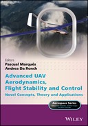
The wind axes system has the xw axis pointing in the wind direction, yw pointing to the right looking into the wind and zw pointing down. With this convention, drag force (D) is in the negative xw direction, side force (S) is in the positive yw direction while lift force (L) is in the negative zw direction, as shown in Figure 5.5.

Figure 5.5 Wind axes frame.
The wind axes force vector Fw in this convention is as follows,
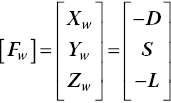
The relationship between the components on the body and wind frames is determined by a transformation matrix [Lbw], as follows,
where [Lbw] is a matrix containing the expressions for converting wind axes forces to body axes forces. For the most common case, a roll angle of zero, [Lbw] matrix components are given by,
where α and β are the attack and yaw angles, respectively.
The moment components on the x, y and z axes are referred to as rolling, pitching and yawing moments, respectively. The moment components in the body axes are the following:

where l, m and n denote moment components with no subscript for body axes.
Moment components on the wind axes are, with subscript w, as follows,
A very common operation is the transfer of force and moment from one point of reference, such as the balance centre (bc), to another reference point, for example the centre of gravity (cg) of the aircraft model. In this case, if a system of force produces a resultant force Fbc and a resultant moment Mbc relative to the balance centre, statics rules indicate that an equivalent system acting at the centre of gravity produces the same force Fcg,
but a different moment Mbc, given by,
where rbc‐cg is the vector from the balance centre to the aircraft centre of gravity.
5.4.2 Instrumentation
Force measurements were carried‐out by using an AB Rollab I6B128 six‐component strain gauge internal balance. The balance is made of high‐tensile steel and every load component is measured by means of a strain gauge bridge. The repeatability of this strain gauge balance is normally better than 0.1% of full scale, but the accuracy of the force measurements depends entirely on the quality of the calibration equipment and evaluation process.
The maximum force measurement range for this balance is,
and the maximum moment measurement range is,

This balance was selected because its range of measurements matches the expected loads on the aircraft model during the test campaign.
During the measurements, the balance is connected to an electric power supply HP 6624. The signal from each bridge of the balance is amplified by a NEC DC Strain Amplifier AS2101. Data acquisition is performed by a National Instruments PXI electronic system. Finally, a computer manages the whole measurement and data acquisition process. Figure 5.6 shows the measurement equipment.

Figure 5.6 Balance‐measurement instrumentation.
Internal balances are usually located inside the aircraft model, so the model is joined to the balance at one end and to the sting at the other. Figure 5.7 shows the balance fixed to the sting support system before the model aircraft was assembled to the balance.

Figure 5.7 Balance fixed to sting support.
5.4.3 Balance Calibration
When subjected to a load, the balance provides a corresponding voltage signal. The relationship between balance output and load input (forces and moments) can be expressed by a second‐order mathematical model as follows [1–4],
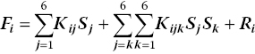
where Fi is the ‘i’ component of the force matrix (i = 1, 2…6), Sj are the balance voltage signals, Kijk are the calibration coefficients and Ri are the residuals. Removing the residuals term, in compact matrix notation,
where [F] is the load vector with six components (three forces and three moments), [S] is the signals matrix with 27 elements and [K] is the calibration matrix (6 rows by 27 columns). The estimation of the calibration matrix is a multiple regression problem, usually solved by applying the least squares method, as follows,
where T and −1 indicate the transposed and inverse matrices, respectively and the matrix [E] is given by,
Prior to the Diana test campaign, the isolated balance was calibrated outside the wind tunnel using the classical load static method. This method is based on the measurement of balance responses when subjected to calibrated loads in order to determine the unknown calibration matrix. For this purpose, a correct calibration requires several loading combinations. Assuming that n loading states are used to calibrate the balance, the corresponding expression is given by,
where matrix subscripts indicate rows × columns.
Additionally, sting deflections are determined by measuring the support deformation when the balance is subjected to loads during the calibration process. Figure 5.8 shows the layout of the rig where the balance is to be calibrated by the classical load static method.
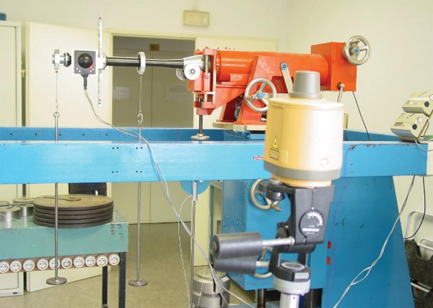
Figure 5.8 Balance calibration layout.
5.4.4 Force and Moment Balance Measurements
The results of the balance measurements are presented in this section as dimensionless coefficients based on a body balance axes system for a maximum wind tunnel airspeed of 50 m/s with zero yaw (β = 0°) and zero roll (ϕ = 0°) angles. The Reynolds number based on the mean aerodynamic chord was 7.5 × 10⁵.
Forces measured by the balance are represented as dimensionless coefficients in the usual manner, as follows,
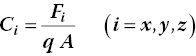
where Fi is the force along the i axis, A is a reference area taken as the wings’ area and q is the dynamic pressure of the air flow defined as q = 0.5ρU∞2, where ρ is the air density and U∞ is the free stream velocity. Aerodynamic coefficients are calculated as a function of the effective AOA, the angle of attack corrected for the sting deflections.
The moment coefficients are defined in analogue form as force coefficients,
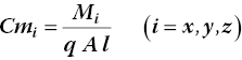
where l is a reference length. Thus, l is the span when i = x, z and the mean aerodynamic chord when i = y.
Results of the force coefficients measurements are depicted in Figure 5.9. The curves show the coefficient Cx being slightly negative up to an AOA of 5°. Above this angle Cx is positive. Coefficient Cz is decreasing with AOA showing a negative slope. Finally, coefficient Cy is zero as expected.

Figure 5.9 Force coefficients versus angle of attack.
Moment coefficients in the balance axes are plotted in Figure 5.10 for the complete aircraft. Coefficients Cmx and Cmz are approximately zero and the pitching moment coefficient Cmy grows with the angle of attack, approximately in a linear form.

Figure 5.10 Moment coefficients versus angle of attack.
5.4.5 Force and Moment in Wind Axes
The results of the balance measurements were transferred from the body axes frame to a more usable wind axis frame. The relationship between the components in the wind and body frames is determined by the following expression,
where [Lbw]T is the transposition of matrix [Lbw], and contains the expressions for converting from the body axes frame to the wind axes frame. For the case for which roll (φ) and yaw (β) angles are zero, [Lbw]T matrix components are given by,

where α is the AOA.
When the wind axes frame is fixed to the centre of gravity of the model and the balance axes frame is fixed to the balance centre, the force relationship is as follows,
Following statics rules, if a system of forces produces a resultant Fw‐bc in the wind axes frame, an equivalent system acting at the centre of gravity produces the same force Fw−cg in the wind axes frame,
Finally, a forces system acting at the centre of gravity of the model expressed in the wind axes frame is given by,

where cg and bc indicate the centre of gravity of the model and the balance centre, respectively.
The wind axes coefficient forces measured are defined as,

where D, S and L are drag, side and lift force, respectively, A is a reference area taken as the wings’ area and q is the dynamic pressure of the air flow defined as q = 0.5ρU∞2, where ρ is the air density and U∞ is the free stream velocity.
Wind axes force coefficients were calculated after transferring the force between frames and the results are shown in Figure 5.11. Lift coefficient CL is increasing with AOA whereas the drag coefficient CD is slowly rising. The side coefficient CS is approximately zero.

Figure 5.11 Force coefficients versus angle of attack (wind axes).
The moment at the centre of gravity is computed from force and moment measured at the balance centre, with all components in wind axes, as follows [1]:
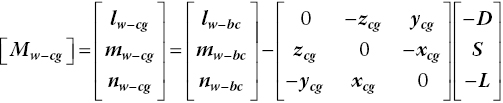
Figure 5.12 shows the transfer of force and moment from the balance centre to the aircraft model centre of gravity. Body axes force is represented on the balance centre (bc) while wind axes force is located at the model centre of gravity (cg).

Figure 5.12 Transference of force and moment from balance centre to centre of gravity.
The pitching moment around the model centre of gravity in wind axes is defined in analogue form as force coefficients:

where c is the mean aerodynamic chord.
Figure 5.13 shows the pitching moment coefficient, which is decreasing as AOA is increasing.
Figure 5.13 Pitching moment versus angle of attack (wind axes).
5.5 Wind Tunnel and CFD Comparisons
This section compares the complete aircraft results calculated using CFD methods and wind tunnel (WT) methods.
5.5.1 Lift Curve
Figure 5.14 shows the curve of the lift coefficient CL as a function of the AOA of the complete aircraft. CFD and WT curves show a linear trend but with slightly different slopes. The maximum WT value of CL is 1.64 at AOA = 18°, corresponding to an overestimated CFD value of CL = 1.85. Lift drop out is observed in the CFD curve above 18° but with a slight recovery from 20°. AOAs higher than 18° were not tested in the wind tunnel due to vibrations of the model giving erroneous balance measurements.
Figure 5.14 Lift curve versus angle of attack.
5.5.2 Drag Curve
The drag curve represents the variation of drag coefficient CD with AOA. Figure 5.15 shows the drag coefficient curve for the complete aircraft using CFD and WT. Both curves show almost the same trend. High coincidence is found when the minimum value of CD = 0.0407 is reached at an AOA of −3.9°. At higher AOAs, the CFD method tends to overestimate the drag force.

Figure 5.15 Drag curve versus angle of attack.
5.5.3 Drag Polar Curve
Drag polar curve represents the drag force coefficient CD versus the lift force coefficient CL taking into account the dependence of both coefficients on the angle of attack. Figure 5.16 shows the drag polar curve of the complete aircraft obtained from CFD and WT. The minimum value of CD can be observed to be coincident in both curves, but slightly different values are obtained when CL is increasing, mainly due to differences between the lift coefficient curves.
Figure 5.16 Drag polar curve.
5.5.4 Pitching Moment Curve
The variation of the pitching moment around the model centre of gravity as a function of AOA is shown in Figure 5.17 by the corresponding dimensionless pitching moment coefficient (Cmcg) versus AOA. Curves from CFD estimates and WT data are sketched in Figure 5.17. They have the same trend with slight differences when the AOA increases. The CFD method underestimates the pitching moment compared to the wind tunnel data. Negative slope (∂Cmcg /∂α < 0) indicates positive static longitudinal stability [5].

Figure 5.17 Pitching moment versus AOA.
Another typical curve, the pitching moment coefficient Cmcg versus the lift coefficient CL is shown in Figure 5.18. The trim point is CL = 0.40 (AOA = 0.55°), corresponding to a zero pitching moment coefficient. This figure shows that CL = 0 gives a pitching moment Cmcg = 0.051. The CFD curve shows an elbow corresponding to stall (AOA = 18°).

Figure 5.18 Pitching moment versus lift.
5.6 Flow Visualization
Flow visualization is a standard non‐intrusive wind tunnel technique that provides qualitative information about the flow‐field topology, giving an interesting picture of the whole‐flow behaviour. In our research, we applied two flow visualization techniques – the surface oil‐film technique and infrared (IR) thermography –to the investigation of the turbojet influence on the tail surfaces.
5.6.1 Oil‐film Technique
The oil‐film technique is based on observations of the flow pattern when a specifically prepared paint is applied to the model surface and when this is illuminated with a UV or similar light source [6–9]. The Diana aircraft model was placed in the wind tunnel test section and painted with a uniform and very thin layer of a mixture of gasoline, oil and a fluorescent pigment in the form of a fine powder. The tunnel was run at the maximum test air speed. The frictional force of the free stream moved the paint and the gasoline evaporated. After turning off, the paint dried into the flow pattern on the model surface, indicating the flow direction, transition, separation, and so on. Enhanced images were obtained, illuminating with black light tubes and digital image recording. The flow visualization was performed at an AOA of 20° and a wind tunnel free stream velocity of 50 m/s. Figure 5.19 shows a view of the fuselage flow visualization.

Figure 5.19 Oil‐film flow visualization on the aircraft fuselage.
Figure 5.20 is a top view of the flow pattern over the left aircraft wing.

Figure 5.20 Oil‐film flow visualization of to the aircraft wing.
Figures 5.21 and 5.22 show a comparison of the flows as calculated from CFD codes and the oil‐film technique. CFD simulations were implemented using the commercial software Fluent 14.5 (ANSYS). Figure 5.21 shows fuselage flow visualization images. The left‐hand picture represents the flow streamlines computed by CFD and the right‐hand side shows the flow from the oil‐film technique. The greyscale version of the image was obtained after brightness and contrast modifications in order to enhance the image quality. The images show good agreement.

Figure 5.21 Fuselage flow visualization: left, CFD; right, oil‐film.
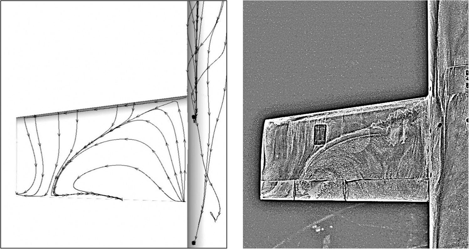
Figure 5.22 Flow visualization over the aircraft wing: left, CFD; right, wind tunnel.
Figure 5.22 shows the aircraft wing flow visualization images. The picture on the left represents the flow streamlines obtained by CFD and that on the right shows the flow visualization obtained by wind tunnel testing (in a greyscale version after brightness and contrast adjustments). Results provided by CFD are close to those given by the oil‐film technique, showing a similar flow pattern, including the separation line.
5.6.2 IR Thermography
Infrared thermography is an experimental technique used to determine the temperature distribution on the model surface. Infrared thermography is based on the remote detection of infrared radiation from objects. This radiation is captured by an IR camera that converts the thermal radiation into a signal video. This gives a measurement of temperature by representing it as a colour temperature map [10]. The objective of the thermography experiment was to investigate the influence of the turbojet exhaust gases over the tail control surfaces. For this purpose, another motorized and reduced‐scale (1:2) Diana model was installed in the wind tunnel test section, supported by a bearing axle located at 1/4 of the wing chord. Figure 5.23 shows the layout of this experiment.

Figure 5.23 Diana aircraft inside the wind tunnel test section.
A Thermovision 900 LW camera from AGEMA Infrared Systems was used for thermal data acquisition. The thermography experiment was carried out at a free stream velocity of 50 m/s with the turbojet engine running to simulate aircraft flight conditions, with hot turbojet exhaust gases arriving at the aircraft tail surfaces. The aircraft was radio controlled during the wind tunnel tests in order to verify the correct behaviour of the aircraft controls.
Figure 5.24 shows the thermography image representing the aircraft in flight with the turbojet running. As can be observed on the image, the turbojet nacelle appears in red whereas orange zones indicate hot regions of the jet flow downstream of the turbojet. Colder regions of the jet are in blue. The IR thermography tests show the flow interaction of the jet with the tail control surfaces, which must be taken into account when determining the flight performance for aircraft operation. In addition, the analysis of thermography images provides information about the real variations of aircraft attitude in AOA as a function of tail control‐surface deflection.

Figure 5.24 Thermography image of the turbojet running.
5.7 Summary and Conclusions
Experimental investigation of the aerodynamics of a new UAV is a classical part of its design process, and it is a fundamental tool in the validation of computational results. An experimental investigation of the Diana UAV was carried out in a low‐speed wind tunnel of the National Institute for Aerospace Technology in Madrid. The results of aerodynamic force and moment measurements were presented by typical dimensionless coefficients. Flow visualizations by the oil‐film technique and IR thermography were also obtained. A comparison of the results from the two methods was performed. This showed that the force computed by CFD generally agrees well with experimental wind tunnel data over a large range, but, the lift, drag, drag polar and pitching moment curves differ at high angles of attack. Flow visualizations of the fuselage and wing surfaces were performed by means of the oil‐film technique. The results are in good agreement with CFD surface streamlines for the fuselage but slight differences appear in the flow over the wing, although the main lines of separation are well predicted by computational techniques. Infrared thermography was used in the wind tunnel testing of a motorized Diana aircraft model. The turbojet was running during the test experiments and the effect of the exhaust gases interacting with the tail surfaces was recorded with the thermography camera. Wind tunnel experiments have a fundamental role in the aerodynamic design process of a general purpose aircraft and can, in many UAV cases, take advantage of the reduced size of the vehicle to use motorized models of the airplane, allowing for a very realistic and accurate description of the aerodynamic characteristics of the UAV.
Acknowledgments
Author wish to acknowledge the support of J.M. Olalla in development of the theoretical and CFD methods that were applied in the aerodynamic design of the Diana UAV. He wish to thank especially S. Sor and M. Urdiales, who were in charge of the Diana wind tunnel experiments, for their collaboration. Last, but not least, our thanks go to all the people involved in the Diana project.
References
- 1 Barlow JB, Rae WH Jr, Pope A 1999 Low‐speed Wind Tunnel Testing, 3rd edn. John Wiley & Sons,.
- 2 Tropea C, Yarin A, Foss JF 2007 Handbook of Experimental Fluid Mechanics. Springer.
- 3 Calibration and use of internal strain‐gauge balance with application to wind tunnel testing. Technical report R‐091‐2003, AIAA, 2003.
- 4 Dubois M 1981 Six‐components strain‐gauge balances for large wind tunnels. Experimental Mechanics: Nov; 401–407.
- 5 Dole CE and Lewis JE 2000 Flight Theory and Aerodynamics, 2nd edn. John Wiley & Sons.
- 6 Merzkirch W 1987 Flow Visualization. 2nd edn. Academic Press.
- 7 Maltby RL 1962 Flow visualization in wind tunnels using indicators. AGARDograph 70. Advisory Group for Aeronautical Research and Development, Paris.
- 8 Goldstein RJ 1996 Fluid Mechanics Measurements. 2nd edn. Taylor & Francis.
- 9 Russo GP 2011 Aerodynamic Measurements. Woodhead Publishing.
- 10 Minkina W and Dudzik S 2009 Infrared Thermography: Errors and Uncertainties. John Wiley & Sons.