8
Aerodynamic Derivative Calculation Using Radial Basis Function Neural Networks
Ranjan Ganguli
Department of Aerospace Engineering, Indian Institute of Science, Bengaluru, India
8.1 Introduction
Aerodynamic stability and control parameters or derivatives are widely used in real‐time simulation, handling qualities analysis and control system design. They play an important role in the development of robotic helicopter UAVs (Kendoul et al 2009; Mokhtari and Benallegue 2004; Mondrag et al 2010). Such helicopters are important for the monitoring of traffic, search and rescue operations, agricultural spraying, logistics and so on (Shakernia et al 1999a,b). Rotorcraft are important unmanned systems due to their capabilities of vertical and low‐speed flight. Several methods of aerodynamic derivative calculation for rotorcraft have been proposed (Agard 1991; Padfield 1999; Prouty 1986). The aerodynamic parameters calculated using the system identification based method are more accurate than those derived from other methods, such as analytical and numerical differentiation (Agard 1991; Padfield 1999). System identification involves reconstructing a simulation model structure and model parameters from experimental flight data. Typical system identification techniques range from simple curve fitting algorithms to complex statistical error analysis.
System identification has become a significant tool for applications such as model validation, handling qualities evaluation, control law design, and flight‐vehicle design and certification (Jategaonkar et al 2004). Estimation and system identification are important problems for rotorcraft micro air vehicles (MAVs). Shen et al (2013) point out that rotorcraft MAVs fly well in 3D environments and can hover in place and maneuver around obstacles. They focus on the problem of estimating the state of rotorcraft MAVs using only onboard cameras and an inertial measurement unit (IMU). They used the pelican quadrotor with an IMU (accelerometer, gyroscope). The vision‐based state estimation onboard the rotorcraft MAV permits autonomous flight. Chowdhary and Jategaonkar (2010) mention that aerodynamic parameter estimation is integral to aerospace system design. They used the unscented Kalman filter (UKF) (Julier and Uhlmann 2004) for aerodynamic parameter estimation of a rotary‐wing UAV from real flight data. The baseline vehicle was the Benda Genesis 1800 helicopter. They used a linear estimation model, which is suitable for rotorcraft in hover (Lorenz and Chowdhary 2005; Mettler 2003). Sensor measurement for all velocities, angular rates and Euler angles were obtained. These measurements are typically corrupted by noise and vibration of the rotorcraft. They concluded that the UKF is a powerful system identification tool.
The methodology and significance of system identification for flight vehicles is available in the literature (Hamel and Kaletka 1997; Hamel and Jategaonkar 2005; Jategaonkar 2006; Morelli and Klein 2005; Tishler and Remple 2006). The system identification method uses techniques such as the maximum likelihood method, equation error method, output error method and filter error method. These methods require a mathematical model of the aircraft with a set of initial values for the parameters to initiate the algorithm (Iliff and Maine 1985, 1986). The identification methods are also affected by the presence of noise, such as state noise or measurement noise (Agard 1991). The identification process becomes more difficult with the increase in the number of degrees of freedom (DoFs) and model parameters. This can happen due to insufficient information content in real‐time flight data (Fu and Kaletka 1993). These problems related to conventional parameter estimation techniques hinder the inclusion of higher‐order DoFs in model development. However, higher‐order modeling is essential for nap‐of‐earth flight, aerial combat, high‐g maneuvers and the design of high‐gain flight control systems (Fu and Kaletka 1993; Pavel 2001). All of these are important issues for unmanned rotorcraft.
New methods for aircraft parameter estimation aim to overcome the shortcomings of classical system identification methods. One such method is the application of artificial neural networks (ANNs) for parameter estimation (Raol and Jategaonkar 1995; Raisinghani et al 1998a,b; Vijaykumar et al 2006). The potential of ANNs has already been demonstrated in fields such as nonlinear flight control, system identification, structural damage detection and identification, flight certification, failure rate prediction and modeling complex phenomena such as ice accretion (Amin et al 1997; Al‐Garni et al 2006; Ganguli et al 1997, 1998; Habib and Zaghloul 1996; Kim and Calise 2005; Malaek and Izadi 2006; Ogretim et al 2006; Reddy and Ganguli 2003; Suresh et al 2005, 2006; Tsou and Shen 1994). Neural networks have been applied to helicopter problems (Horn et al 2002; Kottapalli 2006; Sahani et al 2006). However, the applicability of recurrent neural networks in parameter estimation is limited because of the fixed number of neurons needed for state‐space formulation (Raol and Jategaonkar 1995). In contrast, feed‐forward neural networks (FFNNs) can approximate any measurable function to any desired level of accuracy (Horni et al 1989). This property of FFNNs makes them an ideal choice for aircraft parameter estimation.
To avoid the shortcomings of conventional methods, two new neural network based techniques, the delta method and the zero method, were proposed by Raisinghani and his co‐workers (1998a; 1998b). These methods do not require initial estimates of the parameters; they can be directly extracted from the flight data. Raisinghani’s approach complements existing methods and also has the potential for online parameter estimation. It is based on a type of FFNN known as the multi‐layer perceptron (MLP) which is popular in many applications (Ganguli et al 1998; Suresh et al 2004). However, there are some drawbacks to using MLP, such as the slow convergence rate, computational memory requirements and the sensitivity to outliers. Such difficulties can be avoided by using a different type of FFNN known as radial basis function networks (RBFNs) (Baraldi et al 2000; Park et al 2002; Suresh et al 2004).
Raisinghani et al (1998a) estimated aerodynamic derivatives from simulated fixed‐wing data generated from decoupled lateral and longitudinal modes. This modal decoupling is a reasonable assumption for a fixed‐wing aircraft. For rotary‐wing aircraft, lateral and longitudinal motions are strongly coupled, so the coupled equations of motion should be used to generate simulated data. Raisinghani et al (1998b) also suggested the removal of 25% of estimates from both ends of the ordered set of estimates because of practical problems in parameter estimation in that region This requirement has a negative impact in helicopter problems as it severely effects both transition and the characteristics of the high‐speed flight regime. This drawback of the MLP‐based delta method in derivative computation is overcome by application of RBFN in place of MLP (Kumar et al 2008).
The objective of the present chapter is to outline a methodology for computation of aerodynamic derivatives directly from flight data using RBFN. The proposed approach does not require a mathematical model of the rotorcraft. The delta method using RBFN is first applied to simulated data with added measurement and state noise. The simulated data is generated by a 6‐DoF nonlinear helicopter simulation model, which includes the coupled longitudinal and lateral modes. The method is used to compute derivatives from real time flight test data of the Bo 105 helicopter. The results from the RBFN‐based delta method are compared with the identified derivatives from 6‐DoF and 9‐DoF models available in the literature. The modified 3211 pilot control input is used for rotorcraft parameter estimation. The estimated parameters are then validated from the data generated by a frequency sweep pilot control input, allowing assessment of the predictive capability of the RBFN‐based delta method.
8.2 Helicopter Aerodynamic Derivatives
The helicopter can be mathematically modeled by considering it as a number of subsystems: the main rotor, fuselage, powerplant, empennage, tail rotor and flight control systems (Padfield 1999). The helicopter dynamics are assessed about its center of gravity (cg). An orthogonal axes system is set up with the cg as the origin, as shown in Figure 8.1.

Figure 8.1 Helicopter coordinate system, velocity components and external forces and moments.
We assume that the cg is fixed, even though the rotor blades flap. The equations of motion for this helicopter are derived using physical laws of conservation of momentum and energy and can be expressed as,
With initial conditions ![]() . Here x(t) is a vector of state variables, u(t) is a vector of control variables and f is a nonlinear function. For a 6‐DoF rigid‐body model,
. Here x(t) is a vector of state variables, u(t) is a vector of control variables and f is a nonlinear function. For a 6‐DoF rigid‐body model,
Here, u, v, w are three translational velocity components; p, q, r are three rotational velocity components and ϕ, θ and ψ are Euler’s angles. The function F includes the applied forces and moments that typically emanate from aerodynamic gravitational, inertial and structural sources. The control vector is,
Here θ0, θ1s, θ1c and θtr are the main rotor collective, longitudinal cyclic, lateral cyclic and tail rotor collective. The expanded form of the equations is (Padfield 1999):

Here Ma is the aircraft mass and the moment and products of inertia are (Padfield 1999):

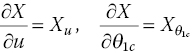
The external forces X, Y, Z and moments L, M, N can be expanded as a Taylor series. For example,

Similar expansions can be obtained for Y, Z, L, M and N. The partial derivative implies that all other state and control variables are held fixed and only one is perturbed. By convention, the derivatives are written as
Using the derivatives, the linearized equation of motion are written as,
where the function f(t) represents disturbances. The system matrix A and control matrix B can be written as

There are 36 stability derivatives and 24 control derivatives for a 6‐DoF model. Some of these are more important than others. Estimation of these derivatives allows us to form a model for developing control algorithms for the unmanned rotorcraft. This chapter presents a general approach for calculating these derivatives.
8.3 Radial Basis Function Neural Networks
Artificial neural networks (ANNs) are a nonlinear function approximation tool that can be used to model complex relationships between the input and output of a system. ANNs can be classified on the basis of the type of connectivity between neurons, type of network architecture and the number of layers in the network. Feed forward neural networks (FFNNs) are composed of several layers of neurons, namely input layer, hidden layer(s) and output layer. Each neuron is connected to others through weights. The training process of FFNNs involves changing the weights to obtain a desired input–output relationship. More details about ANNs of various types is available in Haykins (1994).
Radial basis function networks (RBFNs) are a curve‐fitting method in high‐dimensional space. The basic architecture of RBFNs involves three layers, as shown in Figure 8.2. The input layer contains source nodes. The second layer is the hidden layer, which transforms the input space to a high‐dimensional hidden space. Generally the hidden layer performs a nonlinear transformation. The third layer is made of output neurons, which transforms the hidden space to the output space. Typically, the output neurons perform a linear transformation. The weights in RBFNs exist only between the hidden layer and the output layer. RBFNs are analogous to the Gaussian density function, which is defined by a center position and width parameter. The Gaussian density function is a maximum when the input variables are at the center and decreases monotonically as the distance of the variables from the center increases. The batch mode k‐means clustering algorithm is applied for determining RBFN centers and the weights between the hidden layer and output layer are calculated by the linear least squares optimization algorithm (Haykins 1994). The k‐means clustering algorithm uses the given tracing data to find a set of clusters with each dimensional center. The dimensions of each center are determined by the number of input nodes. This cluster center becomes the center of the RBFN unit.

Figure 8.2 Architecture of radial basis function networks.
The overall input–output mapping can be written as:
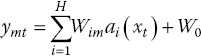
where Gaussian function ![]() is defined as
is defined as

8.4 The Delta Method
The delta method is an ANN‐based approach for parameter estimation. The derivative calculated using this method considers all the data points, thus smoothing noisy data. Derivative calculation by neural network is given by

The neural network is first trained for a particular set of input–output values to create the approximate function ![]() . Then modified input files are prepared in which the variable about which the derivative has to be calculated is perturbed and rest of the inputs are kept constant. These modified input files are then used to calculate derivatives using the trained neural network and the predicted values of outputs are used with the central difference technique. The aerodynamic derivative calculation procedures for fixed‐wing aircraft are given by Raisinghani et al (1998a,b). The practical difficulties faced by those authors at the extremes can be overcome by using RBFNs in place of MLP. As mentioned before, this is necessary for rotorcraft.
. Then modified input files are prepared in which the variable about which the derivative has to be calculated is perturbed and rest of the inputs are kept constant. These modified input files are then used to calculate derivatives using the trained neural network and the predicted values of outputs are used with the central difference technique. The aerodynamic derivative calculation procedures for fixed‐wing aircraft are given by Raisinghani et al (1998a,b). The practical difficulties faced by those authors at the extremes can be overcome by using RBFNs in place of MLP. As mentioned before, this is necessary for rotorcraft.
8.4.1 A Simple Example
The delta method is illustrated by applying it to a simple, single‐input, single‐output, nonlinear function given by
The data is generated for 100 points, in which 50 points are used for training and 50 points for testing of the neural network. Then the delta method is applied to both RBFN and MLP. The number of trainable parameters in both networks is kept identical, to ensure a fair comparison. The derivative is calculated by both RBFN and MLP and the results are compared with the analytical solution given by Eq. (8.5).
It can be seen from Figure 8.3 that the MLP‐based delta method gives an error at the extremes. On the other hand, the RBFN‐based delta method computes the derivative accurately, over the whole range, as shown in Figure 8.4. The effect of noise in the data on derivative computation is also illustrated for this simple function. The noise in the simulated data is added as follows. Assume that we have to include noise in a quantity Y, which is a vector of k elements. The Ynoise is obtained as
where α is the noise level and R is a vector of random numbers between 0 and 1 and has the same size as vector Y.

Figure 8.3 Derivative computation of  using the delta method and multi‐layer perceptron compared with ideal analytical values.

Figure 8.4 Derivative computation of  using delta method and radial basis function network compared with ideal analytical values.
The noise level is kept as 1%. The effect of noisy data on the estimated derivative is shown in Figure 8.5. The direct application of finite difference (FD) method gives substantially more error than derivative computation with the help of the RBFN‐based delta method. Thus the illustrative example clearly shows that the RBFN‐based delta method gives better results at the extremes of the dataset than the MLP‐based delta method. The RBFN‐based delta method is more suitable for rotorcraft parameter estimation, enabling the computation of aerodynamic derivatives in both the transition flight regime and the high‐speed flight regime, which together define the extremes of forward‐speed variation. Moreover, the RBFN‐based delta method gives good results with noisy data, thus making it appropriate for application to real‐time flight test data, which contains noise of varied levels and types. Chowdhary and Jategaonkar (2010) point out that rotorcraft system identification is complicated by noise in measurement and processing due to vibration of the rotorcraft frame and windy conditions. The effect of wind is amplified by the small size of most unmanned rotorcraft. All further results in this chapter are obtained using the RBFN‐based delta method.

Figure 8.5 Derivative computation with delta method (using RBFN) and the FD method and comparison for noisy data.
8.5 Parameter Estimation Using Simulated Data
The 6‐DoF nonlinear helicopter simulation model is based on the DLR Research Bo 105, S123 helicopter. Bo 105 is a lightweight, twin‐engine, multi‐role helicopter with a hingeless rotor. The simulation model used in this work is based on the Level‐1 model and subsystem modeling equations given by Padfield (1981, 1999).
8.5.1 Simulated Data
Simulated flight data for computation of the quasi‐steady aerodynamic derivatives are obtained from a 6‐DoF nonlinear simulation model. The model is trimmed at various forward flight speeds and the forces and moments are obtained at these trim points. Trim involves the solution of the vehicle equilibrium equations of the helicopter. The quasi‐steady aerodynamic derivatives are then obtained using the FD method by numerical perturbation of the state and control variables. The finite difference results are compared with the derivatives estimated using the delta method. The effect of state and measurement noise on both quasi‐steady derivatives is investigated by adding Gaussian noise of varying proportions to the simulated data.
8.5.2 Delta Method to Simulated Data
The simulated data is generated for straight and level flight. The rotorcraft model is trimmed at 70 speed points in the interval (0, 70)m/s and the following trim parameters are computed.
- trim control angles (θ0, θ1c, θ1s, θtr)
- trim forces (X, Y, Z)
- trim moments (L, M, N)
- forward speed (u).
These trim parameters are then used for the derivative computation over a flight range of (0,70) m/s. The derivative computation is done by both the FD method and the delta method. The steps in the delta method are shown in Figure 8.6 and also given below using the Yu stability derivative as an example:
- The input file consists of trim control angles and forward speed.
- The radial basis function network is then mapped with Y force as output.
- Two different modified input datasets with
 are made, keeping the other variables constant.
 - The dataset for
 is presented to the previously trained network and the perturbed output is
  .
. - The dataset for
 is presented to the trained network and the perturbed output is
  .
. - The Yu derivative is computed as
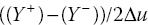 .
.

Figure 8.6 Y u schematic representation of derivative computation using the delta method.
The selection of the number of data points for training is an important aspect in the delta method. We use a training set of 35 data points. The testing set consists of 15 data points, different from the training set.
The delta method is now used to compute some stability and control derivatives. The derivatives are selected keeping in mind the nonlinearities and couplings involved to show that RBFN can capture these effects. The influence of the number of data points on derivative computation is illustrated using Yu derivative computation in Figures 8.7 and 8.8. In both cases, 35 data points are used for derivative computation using the delta method. In Figure 8.7, the FD technique uses the same 35 data points as used in the delta method. Figure 8.8 shows the result when the FD method uses all 70 points of the dataset. Comparing Figures 8.7 and 8.8, it is clear that the FD technique requires more data points for good results. However, the delta method gives good results even with fewer data points. Since flight test data is expensive to obtain and available at few points, the delta method should be used to obtain accurate derivatives in such cases.
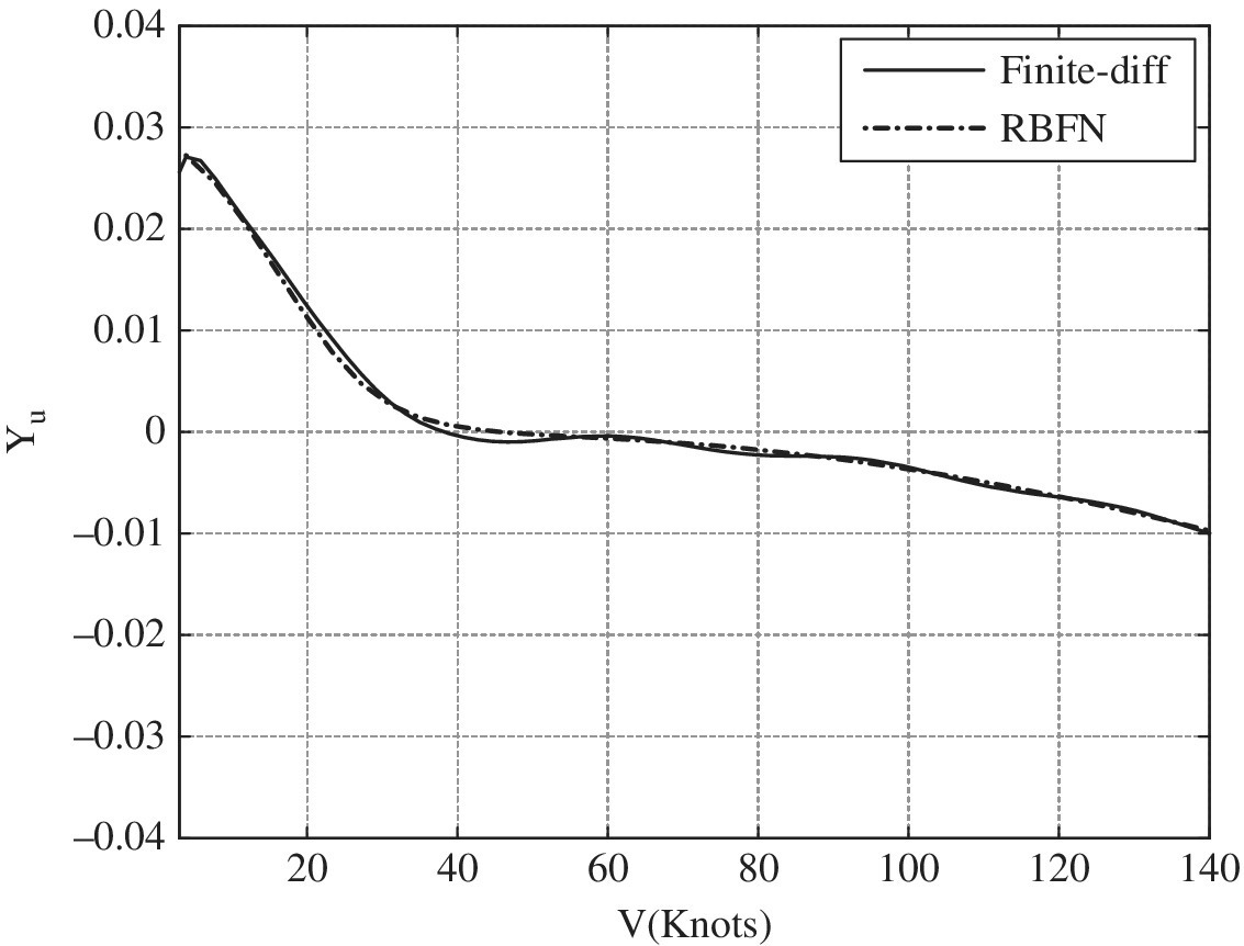
Figure 8.7 Y u stability derivative calculated using delta method with RBFN and FD for 35 data points.
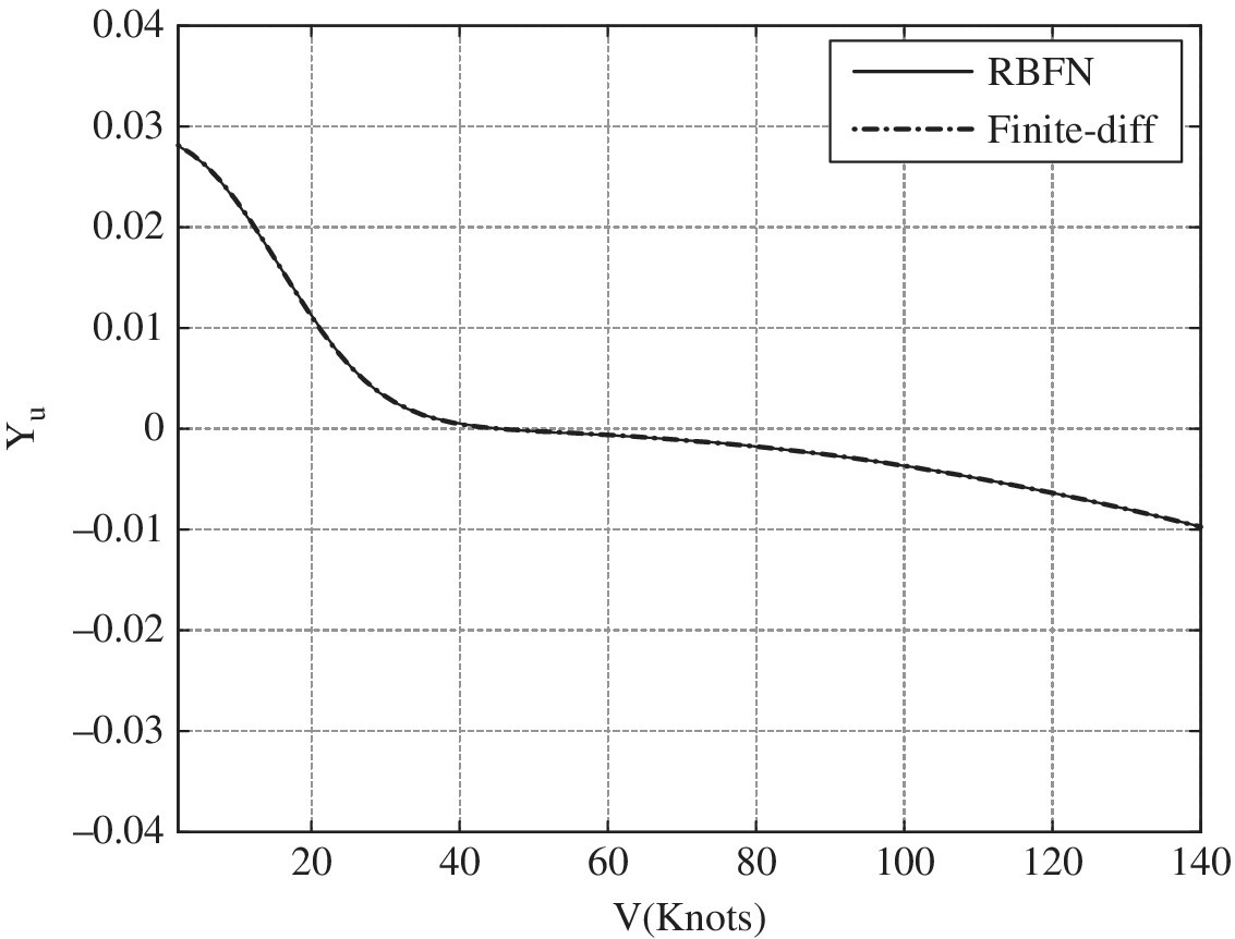
Figure 8.8 Y u stability derivative calculated using RBFN‐based delta method and FD for ideal (zero‐noise) data.
The derivatives are also plotted for 1% measurement noise and state‐noise level for stability derivatives and 5% measurement noise and state‐noise level for control derivatives. Figure 8.9 shows the Yu stability derivative at different forward speeds for noise‐free ideal data. Now Yu is a coupled derivative type and the relatively high value of Yu in low‐speed flight is due to the strong non‐uniform inflow effects in this flight region. This non‐uniform inflow effect reduces with increase in speed, thus making the value of Yu approach zero. In the absence of noise, both the delta and FD derivatives match closely, indicating that the neural network has been properly trained. The effect of measurement and state noise on the Yu derivative is also shown in Figure 8.9. The delta method computes the derivative accurately, whereas the FD approach gives substantial errors. A similar methodology is used to compute the static speed derivative Mu, shown in Figure 8.10.

Figure 8.9 Y u stability derivative calculated using ideal (zero‐noise, finite difference) and noisy data.
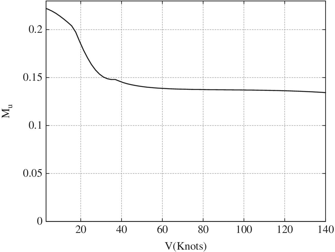
Figure 8.10 M u stability derivative calculated using ideal (zero‐noise) data.
The ![]() control derivative computation using RBFN is given in Figure 8.11. Now
control derivative computation using RBFN is given in Figure 8.11. Now ![]() is an important control derivative, which estimates the heave control sensitivity and quantifies the heave response to the pilot’s main rotor collective input. RBFN successfully computes the control derivative and gives results similar to those obtained from FD for ideal data. As shown in Figure 8.12, the presence of noise in the data deleteriously effects the derivative computation using FD, while the RBFN derivatives closely match the ideal case.
is an important control derivative, which estimates the heave control sensitivity and quantifies the heave response to the pilot’s main rotor collective input. RBFN successfully computes the control derivative and gives results similar to those obtained from FD for ideal data. As shown in Figure 8.12, the presence of noise in the data deleteriously effects the derivative computation using FD, while the RBFN derivatives closely match the ideal case.

Figure 8.11  control derivative calculated using radial basis function network (RBFN) based delta method and finite difference for ideal (zero noise) data.

Figure 8.12
control derivative calculated using ideal (zero noise, FD) and noisy data.
The derivative values are also presented in Tables 8.1 and 8.2 to exemplify the effect of different noise levels on the derivative computation by both FD and RBFN methods. The same levels for both state and measurement noise is used in these comparisons. The comparison uses an error norm between the numerical FD and RBFN outputs both for simulated and noisy data. The derivatives obtained from noisy data by both FD and RBFN techniques are compared with the derivative computed using the FD method from noise‐free simulated data. The error norm is defined as

where X denotes any general force and moment and u is a general state or control variable. Here ![]() is the derivative calculated from either the FD or RBFN methods at a noise level α. Table 8.1 shows the comparison between RBFN and FD for the Yu stability derivative. The error in the derivative calculated by FD increases steadily with increase in the noise level in the simulated data, while the RBFN gives satisfactory output at those higher noise levels. Table 8.2 compares the RBFN and FD results for the
is the derivative calculated from either the FD or RBFN methods at a noise level α. Table 8.1 shows the comparison between RBFN and FD for the Yu stability derivative. The error in the derivative calculated by FD increases steadily with increase in the noise level in the simulated data, while the RBFN gives satisfactory output at those higher noise levels. Table 8.2 compares the RBFN and FD results for the ![]() control derivative.
control derivative.
Table 8.1 Error in the Yu derivative for simulated data with different noise levels.
| Noise level | Method | |
| α(%) | Delta | Finite difference |
| 0 | 0.2260 | 0 |
| 1 | 0.3953 | 1.4016 |
| 3 | 0.6502 | 4.3485 |
| 5 | 0.7638 | 7.7113 |
| 7 | 0.8737 | 9.7445 |
| 10 | 1.0393 | 14.9452 |
Table 8.2 Error in the ![]() derivative for simulated data with different noise levels.
derivative for simulated data with different noise levels.
| Noise level | Method | |
| α(%) | Delta | Finite difference |
| 0 | 0.1043 | 0 |
| 1 | 0.1159 | 0.1388 |
| 3 | 0.1485 | 0.2789 |
| 5 | 0.1611 | 0.3057 |
| 7 | 0.1981 | 0.3481 |
| 10 | 0.2172 | 0.4424 |
To summarize, we see that the quasi‐static aerodynamic derivatives can be calculated accurately using the delta method based on the RBFN neural network. For the ideal or zero‐noise case, the delta method results are almost identical to those obtained using the FD method. Furthermore, the delta method using RBFN does not give any deleterious effects at extreme flight conditions, a problem which haunts the MLP approach. The strength of the delta method is clear when the simulated data is contaminated with state and measurement noise. In such cases, the delta method is robust to noise while the FD method amplifies it. Since rotorcraft data is noisy, the RBFN method is therefore very useful for such vehicles. Since MAV and UAVs are much lighter than full‐scale helicopters, they are prone to noise due to wind gusts and turbulence.
8.6 Parameter Estimation Using Flight Data
Parameter estimation from real‐time flight test data is a complicated process. Conventional parameter estimation methods such as the maximum likelihood estimator need a mathematical model of the system (Chowdhary and Jategaonkar 2010). Such a mathematical model is hard to develop and may not be accurate. The unknown parameters are estimated by exciting the system by a suitable input and then measuring the input and actual system response. The unknown parameters are then computed to ensure that the response of the model to a given input matches the actual response. Mathematical models emanating from system identification are useful for control system design. In general, system identification can be online or offline (Jategaonkar 2006); offline methods need access to the complete set of data. Online methods use data as it becomes available. Recursive system identification is an online method which handles flight data as it becomes available from onboard sensors and calculates the aerodynamic derivatives in real time. Most aerospace systems are nonlinear to some extent and this issue needs to be addressed in system identification.
Unfortunately, model‐based methods become complicated in the presence of noise. Higher‐order modeling also complicates the identification process because the number of parameters is large. The delta method is model‐free and the parameters can be computed directly from flight data.
8.6.1 Flight Test Data
Flight tests with the Bo 105 S123 helicopter were conducted by DLR in 1987 to create a database for system identification. This flight test data is used in this chapter to test the delta method. For flight test data, the helicopter was trimmed in steady‐state horizontal flight at 80 m/s at a density altitude of 915 m. The flight test data includes linear and angular acceleration components, angular rates, linear velocity components, control inputs at the pilot’s stick and rotor blades, along with other variables. The pilot inputs used in the flight tests were:
- positive and negative doublet inputs for each control variable
- positive and negative modified 3211 inputs for each control variable
- pilot‐generated frequency sweeps for each of the four controls.
These inputs were administered to each control individually while the other three controls were kept fixed at their trim values. Details about the flight test input specification are given by Fu and Kaletka (1993). The doublet test input can exite modes in either axis very well, but simple test signals of this type have limitations in a highly coupled rotorcraft model. Doublets are not ideal test inputs for helicopter identification although they may be useful when used in conjunction with other types of input (Agard 1991). In order to alleviate the shortcomings of doublet inputs, a second form of multi‐state input known as the modified 3211 input was developed. The 3211 input excites a wide frequency band within a short period of time, which is suitable for unstable and coupled systems (Agard 1991; Fu and Kaletka 1993). Another form of pilot input known as the frequency sweep is also useful in frequency‐domain rotorcraft identification. The rotorcraft identification problem is difficult to solve using conventional time‐domain techniques due to a high level of measurement noise and the presence of inter‐axis coupling (Fu and Kaletka 1993; Tischler et al 1992, 1985). Fu and Kaletka (1993) applied the modified 3211 input for identification and performed model validation using the frequency sweep input. Similarly, the present study uses data generated by the modified 3211 input for estimation of the parameter. The same input signals as used by Iliff and Maine (1986) are used for identification to ensure a proper comparison of results.
8.7 Delta Method with Flight Data
The flight data is available in terms of linear and angular accelerations. The data is converted to force and moment components by multiplying by the corresponding mass and moment of inertia values, respectively. The modified 3211 signal has a time length of 7 s. Therefore, the parameters are extracted from the data generated for the first 7 s after applying the modified 3211 pilot control. The training dataset is then created to train the RBFN. Each state and control variable is included in the training of the RBFN. This is needed for the mapping of coupling and cross‐axis effects peculiar to rotorcraft. The components of the training set are:
- u, v, w
- p, q, r
- θ0, θ1c, θ1s, θtr
- required force or moment component as output.
First, a training set for a particular stability or control parameter is selected. Then the network is mapped for the given force or moment with the training variables. The input variable about which the derivative has to be computed is perturbed. The rest of the variables are kept unchanged at their original values. The perturbation is made on both the positive and negative sides of the particular input variable. This results in two different datasets: one has a positively perturbed value of the selected state or control variable along with other constant variables and the other has a negatively perturbed value. These modified input datasets are now presented to the trained FBFN. The positive and negative perturbed datasets give the corresponding force or moment perturbed value. The RBFN parameters used are shown in Table 8.3.
Table 8.3 Computational parameters used in RBFN‐based delta method.
| Computational parameters | Value |
| Number of neurons | 234 |
| Spread of radial basis function | 10–35 |
| Δ u | 0.001 m/s |
| Δ v | 0.001 m/s |
| Δ w | 0.001 m/s |
| Δ p | 0.0001 rad/s |
| Δ q | 0.0001 rad/s |
| Δ r | 0.0001 rad/s |
| Δ θ0 | 0.0001 rad |
| Δ θ1c | 0.0001 rad |
| Δ θ1s | 0.0001 rad |
The derivative is then calculated using the central difference formula. The process is illustrated in Figure 8.13 using the Xu derivative as an example. A longitudinal modified 3211 input is used as the pilot input. The steps are:
- Input file is made of all state and control variables.
- The radial basis function network is then mapped with X force as output.
- Two different modified input datasets with
 are made, keeping the other variables constant.
 - The dataset with
 is presented to the previously trained network and the perturbed output is
  .
. - Similarly, the dataset with
 is presented to the trained network and the perturbed output is
  .
. - The Xu derivative can now be computed as
 .
. - The arithmetic mean of Xu computed at all time steps up to 7 s is taken as the final result and is used for comparison with results obtained from conventional techniques.

Figure 8.13 Xu schematic representation of derivative computation using the delta method.
The methodology outlined above is used for computing of all the stability and control derivatives. The derivatives estimated using the delta method are compared with derivatives from the 14‐order model computed by Fu and Kaletka (1993) (see Table 8.4). The parameters estimated by using the RBFN‐based delta method are in the same range as those obtained by the 9‐DoF model.
Table 8.4 Identification results: comparison of delta method and 14‐order model.
| Derivative | Delta method | 14‐order model |
| X u | −0.0340 | −0.0352 |
| X w | −0.0709 | −0.0992 |
| Y v | −0.1245 | −0.1027 |
| Y p | −0.3419 | 1.3823 |
| Z u | −0.0185 | −0.0067 |
| Z w | −0.2646 | −0.2175 |
| Z p | −0.1257 | −0.5669 |
| L u | −0.0833 | −0.0059 |
| L v | −0.1393 | −0.1080 |
| L w | −0.0861 | −0.0683 |
| L q | 0.7040 | 0.5287 |
| M u | −0.0161 | −0.0081 |
| M v | 0.0267 | 0.0281 |
| M w | −0.0181 | −0.0196 |
| M p | −0.7393 | −0.0906 |
| N u | −0.0086 | −0.0039 |
| N v | 0.0781 | 0.1276 |
| N w | 0.0228 | 0.0141 |
| N p | −0.0784 | 0.2973 |
| N r | −1.0738 | −0.8952 |
The computed stability and control parameters are also compared with the identified parameters of the Bo 105 helicopter obtained by researchers at other organizations (see Tables 8.5–8.8; Agard 1991). The delta method estimates most of the stability and control parameters satisfactorily. Since rotorcraft parameter identification from flight test data is an abstruse problem, there is considerable variation in the predictions of different researchers.
Table 8.5 Force derivatives with state variables from delta method and 6‐DoF model.
Source: Agard 1991.
| Derivative | Delta method | AFDD | DLR | Glasgow | NAE |
| Xu | −0.0340 | −0.0385 | −0.059 | −0.032 | −0.050 |
| Xv | −0.0190 | 0* | 0* | 0* | 0.0043 |
| X w | −0.0709 | −0.061 | 0.036 | −0.0422 | −0.017 |
| X p | 0.4166 | 0.756 | 0* | 0* | 0.479 |
| X q | 1.5740 | 2.548 | 0* | 0* | 1.206 |
| Y u | 0.0307 | 0* | 0* | 0* | −0.061 |
| Y v | −0.1245 | −0.221 | −0.170 | −0.131 | −0.279 |
| Y w | −0.1356 | −0.083 | 0* | 0* | −0.0307 |
| Y p | −0.3419 | −2.030 | 0* | 0* | −2.993 |
| Y r | 6.5181 | 0.950 | 1.332 | 0* | 0.807 |
| Z u | −0.0185 | 0.2457 | 0.014 | −0.0883 | 0.1016 |
| Z v | −0.1859 | 0* | 0* | 0* | −0.135 |
| Z w | −0.2646 | −1.187 | −0.998 | −0.791 | −1.106 |
| Z p | −0.1257 | 2.622 | 0* | 0* | 0.385 |
* Eliminated from model structure.
Table 8.6 Moment derivatives with state variables from delta method and 6‐DoF model.
Source: Agard 1991.
| Derivative | Delta method | AFDD | DLR | Glasgow | NAE |
| L u | −0.0833 | −0.061 | −0.081 | −0.027 | −0.099 |
| L v | −0.1393 | −0.207 | −0.271 | −0.098 | −0.270 |
| L w | −0.0861 | 0.168 | 0.116 | 0.130 | 0.116 |
| L p | −4.1502 | −8.779 | −8.501 | −4.470 | −1.895 |
| L q | 0.7040 | 3.182 | 3.037 | 0* | 4.454 |
| L r | 0.9065 | 0.991 | 0.410 | 1.318 | 0.434 |
| M u | −0.0161 | 0* | 0.029 | 0.0203 | 0.0078 |
| M v | 0.0267 | 0.050 | 0.048 | 0* | 0.0248 |
| M w | −0.0181 | 0.096 | 0.053 | 0.0491 | 0.0696 |
| M p | −0.7393 | −0.998 | −0.419 | −1.367 | −1.414 |
| M q | −2.3217 | −4.493 | −3.496 | −2.217 | −2.992 |
| N v | 0.0781 | 0.082 | 0.117 | 0.0784 | 0.112 |
| N w | 0.0228 | −0.119 | 0.034 | 0.0281 | −0.0634 |
| N p | −0.0784 | −0.466 | −1.057 | −1.302 | −0.692 |
| N r | −1.0738 | −1.070 | −0.858 | −0.756 | −1.017 |
* Eliminated from model structure.
Table 8.7 Force derivatives with control variables from delta method and 6‐DoF model.
Source: agard.
| Derivative | Delta method | AFDD | DLR | Glasgow | NAE |
|
|
0.0319 | −0.046 | 0* | 0* | −0.0222 |
|
|
−0.0268 | −0.072 | −0.028 | −0.048 | −0.05 |
|
|
−0.0063 | 0* | 0* | 0* | −0.00176 |
|
|
−0.0309 | −0.032 | 0* | 0* | −0.0152 |
|
|
−0.2841 | −0.388 | −0.349 | −0.259 | −0.337 |
|
|
−0.1371 | −0.103 | −0.303 | −0.140 | −0.175 |
* Eliminated from model structure.
Table 8.8 Moment derivatives with control variables by delta method and 6‐DoF model.
Source: Agard 1991.
| Derivative | Delta method | AFDD | DLR | Glasgow | NAE |
|
|
0.0130 | 0.058 | 0.032 | 0* | 0.0142 |
|
|
0.0243 | 0.073 | 0.024 | 0* | −0.005 |
|
|
0.0392 | 0.179 | 0.185 | 0.0764 | 0.1361 |
|
|
0.0292 | 0.073 | 0.057 | 0.039 | 0.048 |
|
|
0.0470 | 0.098 | 0.093 | 0.0565 | 0.0787 |
|
|
−0.017 | 0* | −0.009 | 0* | 0.0106 |
|
|
−0.0104 | −0.051 | 0* | 0* | −0.036 |
|
|
−0.0436 | −0.075 | 0* | 0* | −0.051 |
|
|
0.0318 | 0.033 | 0.026 | 0* | 0.047 |
* Eliminated from model structure.
Verification is an important step in the system identification process. Verification should be conducted with data not used in identification. Therefore, flight test data from frequency sweeps are used for the verification. Tables 8.9–8.11 compare estimated derivatives from modified 3211 and frequency sweep pilot control inputs. There is good agreement in direct and coupled stability derivatives, demonstrating the predictive capability of the delta method.
Table 8.9 Verification of force derivatives using frequency sweep input.
| Derivative | 3211 | Frequency sweep |
| X u | −0.0340 | −0.0373 |
| X v | −0.0190 | −0.0117 |
| X w | −0.0709 | −0.0566 |
| X p | 0.4166 | 1.09 |
| X q | 1.5740 | 1.2188 |
| Y u | 0.0307 | 0.0444 |
| Y v | −0.1245 | −0.1143 |
| Y w | −0.1356 | −0.1835 |
| Y r | 6.5181 | 6.4246 |
| Z u | −0.0185 | −0.0263 |
| Z v | −0.1859 | −0.1987 |
| Z w | −0.2646 | −0.3169 |
Table 8.10 Verification of moment derivatives using frequency sweep input.
| Derivative | 3211 | Frequency sweep |
| L u | −0.0833 | −0.0425 |
| L v | −0.1393 | −0.0179 |
| L w | −0.0861 | −0.0210 |
| L q | 0.7040 | 2.4766 |
| M u | −0.0161 | −0.0327 |
| M v | 0.0267 | 0.0527 |
| M w | −0.0181 | −0.0133 |
| M p | −0.7393 | −0.5531 |
| N u | −0.0086 | −0.004 |
| N v | 0.0781 | 0.1326 |
| N w | 0.0228 | 0.0376 |
| N p | −0.0784 | −0.5635 |
| N r | −1.0738 | −1.0872 |
Table 8.11 Verification of control derivatives using frequency sweep input.
| Derivative | 3211 | Frequency sweep |
|
|
0.0319 | 0.0304 |
|
|
−0.0268 | −0.0237 |
|
|
−0.0309 | −0.0407 |
|
|
−0.2841 | −0.3778 |
|
|
−0.1371 | −0.094 |
|
|
0.0130 | 0.0172 |
|
|
0.0392 | 0.583 |
|
|
0.0243 | 0.0208 |
|
|
0.0292 | 0.0317 |
|
|
0.0470 | 0.0545 |
|
|
−0.0107 | −0.0093 |
|
|
0.0318 | 0.0271 |
The RBFN approach is philosophically different from the other classical system identification approaches. The RBFN‐based delta method is model‐free and therefore provides a useful tool for rotorcraft parameter identification from flight test data. RBFN‐based derivatives can also be used to compare to derivatives obtained using conventional system identification techniques.
8.8 Summary
Rotorcraft parameter estimation based on the RBFN‐based delta method has been discussed. This technique is model‐free and is suitable for rotorcraft UAVs and MAVs. The method is first evaluated on simulated data generated by a nonlinear simulation model. Both ideal (noise free) and noise‐contaminated data are considered. Both state and measurement noise are considered. Then the approach is used to compute the stability and control derivatives directly from real time flight test flight data of a Bo 105 helicopter.
The RBFN is able to successfully map the coupling and nonlinearities in the system and estimate satisfactory stability and control derivatives using the delta method, both for simulated ideal and noisy data. The delta method is robust to noise present in the data. The performance is satisfactory in case of state and measurement noise. The delta method identifies the parameters from flight data and the results have about the same level of accuracy as a 14‐order model. The delta method gives satisfactory results for sparse data points. This helps in parameter estimation when the fewer data points are obtained from flight tests. Parameter estimation using RBFN has acceptable predictive capability: the verification results from frequency sweep input are in the same range as those estimated using a modified 3211 input. The RBFN approach provides an alternative to the conventional parameter identification approach when a mathematical model is not available. It can also be used as a method that gives an estimate of the derivatives, which can be used to guide conventional parameter estimation work and model development.
Acknowledgements
The author thankfully acknowledges Dr R. Jategaonkar and Dr W.V. Gruenhagen, DLR, Germany, for providing the Bo 105 flight data. He also acknowledges his research collaborator Dr S.N. Omkar and his former students Dr. M. Vijaya Kumar and Mr. Rajan Kumar.
References
- Agard1991agard Agard 1991 Rotorcraft system identification, Technical Report AR 280, LS 178, Advisory Group for Aerospace Research & Development.
- Amin SM, Gerhart V and Rodin EY 1997 System identification via artificial neural networks – applications to on‐line aircraft parameter estimation, SAE Transactions, 106, 1787–1808.
- Al‐Garni AZ, Jamal A, Ahmad AM, Al‐Garni AM and Tozan M 2006 Failure‐rate prediction for De Havilland Dash‐8 tires employing neural network technique, Journal of Aircraft, 43 (2), 537–543.
- Baraldi A, Blonda P, Satalino G, D’Addabbo A and Tarantino C 2000 RBF two stage learning networks exploiting supervised data in the selection of hidden unit parameters; an application to SAR data classification, Proceedings in IGARSS, Honolulu, HI, pp. 672–674.
- Chowdhary G. and Jategaonkar R. 2010 Aerodynamic parameter estimation from flight data applying extended and unscented Kalman filter, Aerospace Science and Technology, 14 (2), 106–117.
- Fu KH and Kaletka J 1993 Frequency domain identification of Bo105 derivative models with rotor degrees of freedom, Journal of American Helicopter Society, 38 (1), 73–83.
- Ganguli R, Chopra I and Haas DJ 1997 Detection of helicopter rotor system simulated faults using neural networks, Journal of American Helicopter Society, 42 (2), 161–171.
- Ganguli R, Chopra I and Haas DJ 1998 Helicopter rotor system fault detection using physics‐based model and neural networks, AIAA Journal, 36 (6), 1078–1086.
- Hamel PG and Kaletka J 1997 Advances in rotorcraft system identification, Progress in Aerospace Sciences, 33 (4), 259–284.
- Hamel PG and Jategaonkar RV 2005 Evolution of flight vehicle system identification, Journal of Aircraft, 33 (1), pp. 9–28.
- Habib S and Zaghloul ME, System identification using time dependent neural networks – a simpler approach, AIAA Guidance, Navigation, and Control Conference, San Diego, CA. AIAA Paper 1996–3803
- Horn J, Calise AJ and Prasad JVR 2002 Flight envelope limit detection and avoidance for rotorcraft, Journal of American Helicopter Society, 47 (4), 253–262.
- Horni KK, Stinchcombe M and White H 1989 Multi‐layer feed forward networks are universal approximaters, Neural Networks, 2 (5), 359–368.
- Haykin S 1994 Neural Networks: A Comprehensive Foundation, Macmillan.
- Iliff KW and Maine RE 1985 More than you may want to know about maximum likelihood estimation, Technical report TM 85905, NASA.
- Iliff KW and Maine RE 1986 Application of parameter estimation to aircraft stability and control the output error approach, Technical report RP 1168, NASA.
- Jategaonkar RV, Fischenberg D. and Gruenhagen WV 2004 Aerodynamic modeling and system identification from flight data – Recent applications at DLR, Journal of Aircraft, 41 (4), 681–691.
- Julier SJ and Uhlmann JK 2004 Unscented filtering and nonlinear estimation, Proceedings of the IEEE, 92 (3), 401–422.
- Jategaonkar RV 2006 Flight Vehicle System Identification: A Time Domain Methodology, AIAA.
- Kendoul F, Kenzo N, Isabelle F. and Rogelio L 2009 An adaptive vision‐based autopilot for mini flying machines guidance, navigation and control, Autonomous Robots, 27 (3), 165–188.
- Kim BS and Calise AJ 2005 Nonlinear flight control using neural networks, Journal of Guidance, Control, and Dynamics, 20 (1), 26–33.
- Kottapalli S 2006 Neural network modeling of UH‐60A pilot vibration, Journal of American Helicopter Society, 51 (2), 195–201.
- Kumar R. and Ganguli R. and Omkar SN and Kumar MV 2008 Rotorcraft parameter identification from real time flight data, Journal of Aircraft, 45 (1), 333–341.
- Lorenz S and Chowdhary G 2005 System identification for a miniature rotorcraft, Preliminary Results, AHS 61st Forum, Grapevine, TX.
- Malaek SMB. and Izadi HA, 2006 Progressive certification process based on living systems architecture using learning capable controllers, Journal of Aircraft, 43 (1), 207–215.
- Mettler B 2003 Modeling Identification and Characteristics of Miniature Rotorcrafts, Kluwer Academic Publishers.
- Mokhtari A and Benallegue A 2004 Dynamic feedback controller of Euler angles and wind parameters estimation for a quadrotor unmanned aerial vehicle, Proceedings of IEEE International Conference on Robotics and Automation, Vol. 3, pp. 2359–2366.
- Mondragón IF, Olivares‐Méndez MA, Campoy P, Martínez C and Mejias L 2010 Unmanned aerial vehicles UAVs attitude, height, motion estimation and control using visual systems, Autonomous Robots, 29 (1), 17–34.
- Morelli EA and Klein V 2005 Application of system identification to aircraft at NASA Langley Research Center, Journal of Aircraft, 42 (1), 12–25.
- Ogretim E, Huebsch W and Shinn A 2006 Aircraft ice accretion prediction based on neural networks, Journal of Aircraft, 43 (1), 233–240.
- Padfield GD 1981 A theoretical model of helicopter flight mechanics for application to piloted simulation, Technical report 81048, RAE.
- Padfield GD 1999 Helicopter Flight Dynamics: The Theory and Application of Flying Qualities and Simulation Modeling, AIAA.
- Pavel M 2001 On the necessary degrees of freedom for helicopter and wind turbine low‐frequency mode modeling, PhD Thesis, Technische Universiteit Delft.
- Park JW, Harley RG and Venayagamoorthy GK 2002 Comparison of MLP and RBF neural networks using deviation signals for on‐line identification of a synchronous generator, IEEE Power Engineering Society Winter Meeting, 1, 274–279.
- Prouty RW 1986 Helicopter Performance, Stability, and Control, Krieger Publishing.
- Raol JR and Jategaonkar RV 1995 Aircraft parameter estimation using recurrent neural networks‐a critical appraisal, 20th Atmospheric Flight Mechanics Conference. AIAA Paper 95–3504.
- Raisinghani SC, Ghosh AK and Kalra PK 1998a Two new techniques for parameter estimation using neural networks, The Aeronautical Journal, 102 (1011), 25–29.
- Raisinghani SC, Ghosh AK and Khubchandani S 1998b Estimation of aircraft lateral‐directional parameters using neural networks, Journal of Aircraft, 35 (6), 876–881.
- Reddy RRK and Ganguli R 2003 Structural damage detection in a helicopter rotor blade using radial basis function neural networks, Smart Materials and Structures, 12 (2), 232–241.
- Sahani NA, Horn JF, Jeram GJJ and Prasad JVR 2006 Hub moment limit protection using neural network prediction, Journal of American Helicopter Society, 51 (4), 331–340.
- Shakernia OMY, Koo TJ and Sastry S 1999 Landing an unmanned air vehicle: Vision‐based motion estimation and nonlinear control, Asian Journal of Control, 1 (3), 128–145.
- Shakernia O, Ma Y, Koo TJ, Hespanha J and Sastry SS 1999 Vision guided landing of an unmanned air vehicle, Proceedings of the 38th IEEE Conference on Decision and Control, Vol. 4, pp. 4143–4148.
- Shen S, Mulgaonkar Y, Michael N and Kumar V 2013 Vision‐based state estimation for autonomous rotorcraft MAVs in complex environments, IEEE International Conference on Robotics and Automation, pp. 1758–1764.
- Suresh S, Omkar SN, Mani V and Sundararajan N 2005 Nonlinear adaptive neural controller for unstable aircraft, Journal of Guidance, Control, and Dynamics, 28 (6), 1103–1111.
- Suresh S, Omkar SN, Mani V and Sundararajan N 2006 Direct adaptive neural flight controller for F‐8 fighter aircraft, Journal of Guidance, Control, and Dynamics, 29 (2), 454–464.
- Suresh S, Omkar SN, Ganguli R and Mani V 2004 Identification of crack location and depth in a cantilever beam using a modular neural network approach, Smart Materials and Structures, 13 (4), 907–915.
- Tishler MB and Remple RK 2006 Aircraft and Rotorcraft System Identification: Engineering Methods WITH Flight‐Test Examples, AIAA.
- Tsou P and Shen MHH 1994 Structural damage detection and identification using neural networks, AIAA Journal, 32 (1), 176–183.
- Tischler MB and Cauffman MG 1992 Frequency‐response method for rotorcraft system identification: flight applications to Bo105 Coupled rotor/fuselage dynamics, Journal of American Helicopter Society, 37 (3), 3–17.
- Tischler MB, Leung JGM and Dugan DC 1985 Frequency‐domain identification of XV‐15 tilt‐rotor aircraft dynamics in hovering flight, Journal of American Helicopter Society, 30 (2), 38–48.
- Vijaykumar M, Omkar SN, Ganguli R, Sampath P and Suresh S 2006 Identification of helicopter dynamics using recurrent neural networks and flight data, Journal of American Helicopter Society, 51 (2), 164–174.