
2.1 Scope
As the name implies, this book covers only the basic application of NEC-2 to the design and analysis of MF directional antennas. The essentials are described in sufficient detail to teach the useful design and analysis of medium-frequency (MF) broadcast antenna arrays, but some refinements of NEC-2 are not specifically described in this text or they are given only cursory mention. Some of these refinements include the use of symmetry and reflection to simplify the input file, wire arcs, dimension scaling, and multiple structures. Only a cursory explanation of the use of Numerical Green's Function and the Sommerfeld/Norton finite-ground method is given in the last chapter so more study will be needed to fully exploit those topics.
In addition, NEC-2 has some capabilities that are not usually associated directly with broadcasting; therefore, those topics are not included in this text. These include the ability to model helix and cylindrical structures, surface patches, and circular and elliptical polarization.
However, to augment the material in the text, Appendix A includes the complete catalog of NEC-2 commands. They are described in sufficient detail in the appendix to permit the reader to individually extend study to any capability of NEC-2.
2.2 The NEC-2 Engine
The Numerical Electromagnetics Code was written in 1977 by G. J. Burke and A. J. Poggio at Lawrence Livermore National Laboratory under contract to the U.S. Navy. The code was originally known as the Numerical Electromagnetics Code (NEC). As the code was improved over time, it was renamed NEC-2 in 1980, NEC-3 in 1983, and ultimately NEC-4 in 1990. NEC-2 has been declared public domain, NEC-3 no longer exists, and the distribution of NEC-4 is controlled by licensing through the Industrial Partnership and Commercialization Office at Lawrence Livermore National Laboratory.
The NEC-4 source code is an extensive revision of the NEC-2 code that makes more use of the Fortran 77 constructs and is more modular and easier to understand and maintain. Additional features and capability were added in the revision process. For example, NEC-2 models wire structures both in free space and over a ground plane. The ground plane may be either perfectly conducting or have finite ground characteristics. NEC-4 possesses the same abilities as NEC-2 in this regard plus it is able to model wire structures buried in the ground or passing through the air/ground interface.
NEC-4 also carries revisions of the NEC-2 code that reduce the loss of precision when modeling tightly coupled wires and electrically small structures. In addition, NEC-4 has been changed to be more accurate than NEC-2 when treating models containing stepped-radius wires or junctions of wires of differing radius. NEC-4 can also accommodate the effects of insulated wires, whereas NEC-2 has no such provision.
Thus, while NEC-4 is, indeed, considered the most accurate, NEC-2 is quite adequate for most broadcast applications. Therefore, because NEC-2 is in the public domain and available at no charge, it was selected to be the code used in this book.
Both the executable and source code for NEC-2 are widely distributed on the Internet and the code has been liberally modified by various users. The NEC-2 computer program used in this book is a modified version of NEC2dxs.zip. At the time of this writing, NEC2dxs.zip can be downloaded free of charge from the Internet: http://www.si-list.net/swindex.html.
The unzipped version has been included on the disk that accompanies this book. What's there has been modified and renamed bnec .exe but will be referred to henceforth by the general term NEC-2. The program bnec.exe is a Win 95/98/Me/NT4/2000/XP 32 bit Windows application that works from a DOS console window. It has been modified slightly to make the GM command input format more useful to the broadcaster and to dimension the arrays to accommodate a 120 wire ground screen. It has also been changed to protect the input file from accidental erasure. Please be aware that the GM command (described in Chapter 3) has been modified. It is compatible with bnec.exe, but the modified version is not compatible with the usual NEC2dxs programs. The GM command used here is, however, compatible with the NEC-4 file format. Therefore, the input files generated during the study of this book are, for the most part, usable with both bnec.exe and NEC-4.
2.3 NEC-2 Operation
In perhaps an oversimplified explanation, the antenna to be analyzed is modeled by a series of wires and voltage sources as described to NEC-2 in an input file furnished by the user. When run, NEC-2 divides each wire into the number of segments specified by the user. It then calculates the current on each segment and finally sums the effects of all segments to get a final result. NEC-2 stores its output in a file that it places in the computer's currently active folder. The user must recall the output file to read, print, or otherwise use it.
2.4 Creating the Input File
To use NEC-2, the user must generate an input file that describes the antenna geometry and operating parameters in a defined format. This is done using any convenient text editor and saving the file in text form. When NEC-2 is run, it issues a call for the path and name of the input file plus the name that the user wishes to assign to the output file. There are no other communications with the user while NEC-2 runs.
2.4.1 Naming the Files
During the course of conducting a directional array analysis, it is necessary to make several NEC-2 runs and to generate several NEC-2 input and output files. To conveniently keep track of the various files, a naming convention is recommended. The convention used in this book is defined as we go along and the reader is encouraged to follow that convention to avoid confusion.
In that regard, it is sufficient to say at this time that all files may be named with the call letters of the station using the antenna array. For some discussions in this book, CALL will represent a generic station call being used for illustration purposes. All input files will carry the extension .NEC. Thus, the input file will be named CALL.NEC. The output file generated by NEC-2 when CALL.NEC is the input file can be named anything but it is highly recommended that it be named CALL.OUT.
2.4.2 Data Commands
The original NEC-2 computer program used punched cards to input the data that describes an antenna and to request computation of antenna characteristics. But, as mentioned earlier, modern NEC-2 now uses an input text file with the format of the data within that file being similar to that of the punched card set. Each line in the input file is a separate command and each command carries the data that initially appeared on a single punched card. Instead of the data being written into positional fields, however, modern NEC-2 files use data fields delimited by commas or spaces. Because of the similarity to a punched card set, and of course the inertia of habit, each data statement command in the input file is sometimes referred to as a “card.” However, in an attempt to be more descriptive, this book follows the precedent set by the documentation of NEC-4 and uses the word “command” rather than the word “card” when referring to the statements in the input file.
A typical data command is:
The commands in an input file must be written in ASCII text and they must begin in column 1 of line 1. Each successive command must then begin in column 1. Do not indent the commands or use spaces at the beginning of the commands and do not use blank lines.
Every data command begins with a two-letter alphabetic code in columns 1 and 2 to identify the command to the program. There are 34 two-letter command codes in the NEC-2 vocabulary and all of them are given in Appendix A. However, only about 20 of these codes are normally used in broadcast calculations. The simple example that follows later uses only 9 of the command codes and those are probably the most common command codes used by broadcasters.
All commands having numeric data are written in a similar format, with fields for integer numbers first, followed by fields for real numbers. Integer numbers are written with no decimal point. Real numbers are written as a string of digits and may contain a decimal point. Real numbers may also be written as a string of digits containing a decimal point followed by an exponent of 10 in the form 1.234E±6. This is interpreted as multiplying the number 1.234 by 10±6.
2.4.3 Data Command Types
The input file for a single NEC-2 run must contain at least one of each of the three types of command.
- The input file must begin with one or more comment commands that can contain any type of information but they usually provide a description of the NEC-2 run. This information is printed at the start of the output file as a label.
- The comments are followed by geometry commands, which describe the antenna system. The geometry commands have two fields for integer numbers followed by real-number fields as necessary.
- Finally, a number of program control commands specify electrical parameters such as frequency, loading, and excitation. Commands of this type also request the execution of the .NEC file. The program control commands have four integer fields followed by realnumber fields.
2.4.4 An Input File Illustration
The following illustration is included here to stimulate the reader's interest before we embark upon a series of long explanations. A single tower is used in this example because it is the simplest representation. Of course, a broadcast array will have multiple towers. The object of this one-tower calculation might be to determine the driving point impedance of the tower, although enough data is included in the output file to enable one to plot the current distribution on the tower and to view the antenna radiation pattern.
Remember that the data commands in an input file must begin in column 1 of line 1. Each successive command must then begin in column 1. Do not indent the commands or use spaces at the beginning of the commands and do not use blank lines.
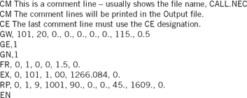
The example input file listed here contains three comment commands (CM, CM, CE), two geometry commands (GW, GE), and five program control commands (GN, FR, EX, RP, EN). A full explanation of all the input commands is given in Appendix A. As each command code is addressed in the paragraphs that follow, the reader is encouraged to read the full description of that command code as it appears in Appendix A.
The commands in Listing 2-1 make up the sample input file.
Comment Commands
Every input file must contain at least one comment command and if there is only one comment command, it must be the CE command. Any other comment commands must precede the CE command and must be identified as CM commands. In the preceding example. CM and CE are comment commands.
Geometry Commands
Several types of geometry command can be used to describe the wires in an antenna but the GW is the most used for broadcast work. The
Listing 2-1
GW command describes a straight wire located in an XYZ coordinate system where lengths are measured in meters. For our broadcast work, towers are considered to be wires or to be made up of a group of wires. The simplest description of an antenna tower is a single vertical wire of defined radius, as represented in the GW command of Listing 2-1.
The position of each wire must be specified and the number of segments into which the wire is to be divided must also be specified. The position of a wire is defined by showing the coordinates of each end, as presented in the XYZ coordinate system. While you must specify the number of segments, it is not necessary to define the position of each segment because NEC-2 does this routinely. While only one wire is used in the simple example above, multiple wires can be used to describe a single tower and, of course, multiple wires are used to describe a multitower directional array.
Referring to the GW wire in Listing 2-1, the number 101 is the wire tag number assigned to identify this wire. By broadcast convention, the 100 tag series (101, 102, 103, etc.) is used to identify wires associated with tower 1. The 200 series (201, 202, 203, etc.) identifies wires associated with tower 2; the 300 series, tower 3, and so on. Be sure to get into the habit of using this convention because some postprocessing programs take advantage of this convention to identify towers and to determine the number of towers in an array.
In Listing 2-1, the wire tag 101 in the GW command shows that this is wire 1 of tower 1. Next, the digits 20 show that we have elected to divide the wire into 20 segments. The next three fields show that the first end of the wire is located at X = 0 meters, Y = 0 meters, and Z = 0 meters (ground level at the origin). The following three fields show that the second end of the wire is located at X = 0 meters, Y = 0 meters, Z = 115 meters. This describes a vertical tower (wire) located at the origin and 115 meters high. The last field of the GW command shows that the effective radius of the tower is defined to be 0.5 meters.
Next is the GE command, which is mandatory and indicates the end of the geometry description. The GE command also signals whether the antenna is in free space or whether it is operating over a ground plane. GE with no following digit, or with the digit 0 following, indicates free space operation, whereas GE with the digit 1 following is used when a ground plane is present. The GE command does not specify the characteristics of the ground plane; it only readies NEC-2 to accept the ground-plane parameters from a following command. If a ground plane is present, then in addition to the GE command, the GN command must be included to define the characteristics of that ground plane. Please read the full description of the GE command and the GN command in Appendix A.
Program Control Commands
The GN command is a program control command and shows the characteristics of the ground in the immediate vicinity of the antenna. Appendix A explains that the digit 1 following GN shows that the ground plane is perfectly conducting. A zero or 2 following GN indicates a finitely conducting ground, which must be defined in the remaining fields of the GN command. The finitely conducting ground is used only in calculating radiated fields. The NEC-2 calculated value for the self-impedance of the tower will be the same whether using a perfecting conducting ground or a ground with finite constants. Please refer to appendix A for more details on the GN command.
The FR command sets the frequency to 1.5 MHz, although it is capable of doing more. See Appendix A for a full description of the use of the FR command.
The first zero on the EX command shows we are exciting the wire with a voltage source. The following two data fields showing wire tag 101 and segment 1 place the excitation on wire 1 of tower 1 using segment 1. The excitation is defined to be 1266.084 + j0 volts by the last two fields of the EX command. Notice that the excitation voltage is a complex number expressed by its real and imaginary parts; thus, it has both magnitude and phase.
It is important to say here that modeling voltage sources is a critical step in the analysis of broadcast antennas. NEC-2 offers two models for voltage sources, the applied-field source and the bicone source. The applied-field source (I1 = 0 on the EX command) is most appropriate for broadcast work. See the EX command in Appendix A for a full explanation.
The RP command tells NEC-2 to calculate the radiated pattern. This command is also an automatic execute command. The XQ command can also be used to cause execution but it is not necessary when preceded by the RP command, although no error is caused if the XQ command is included. Again, refer to Appendix A to read the full description of each of these commands.
As an exercise, type the input file commands given as Listing 2-1 in Section 2.4.4 into a file and save it as a text file with the name CALL.NEC. Any convenient text editor may be used—the EDIT command in Windows works fine, as does WordPad and Notepad. If WordPad or Notepad is used, be sure to save the work as a text file.
2.5 Reading the Output File
To run the CALL.NEC input file using bnec.exe, place CALL.NEC and bnec.exe in the same folder, then run bnec.exe. The bnec.exe will ask for the name of the input file, which is CALL.NEC. It will then ask for the name that you wish to assign to the output file, and an appropriate response is CALL.OUT. When bnec.exe finishes its run, it will leave the output file (CALL.OUT) in the currently active folder.
If your input file contains an error, NEC-2 does not signal that error during the run time. Instead, it records the error in the output file and aborts the run if it is a fatal error. Therefore, you must examine the output file to identify an error. A brief description of the error will appear at the place in the output file where the error occurred. More error descriptions are given in general in Appendix B.
The output file can be quite long and it contains some lines longer than 100 characters; thus, it is difficult to read in a DOS window. The output file is most conveniently viewed using WordPad and called by a batch file whose location is included in the PATH variable of the AUTOEXEC.BAT file. While on this subject, it is recommended that you also include bnec.exe and a viewing program (described in Appendix C) called NVCOMP.EXE in the PATH variable of the AUTOEXEC.BAT file. This will make it more convenient for you to make calculations from any folder.
A satisfactory hard copy of the output file can be printed in the portrait orientation by changing the font of the entire file to size 6. The font can be changed to size 8 if the file is printed in the landscape orientation. (Listings and outputs are shown in 8.5 point Trade Gothic font throughout this book.)
Portions of the file CALL.OUT are displayed next with commentary. Please refer to your own printout if you have made one.
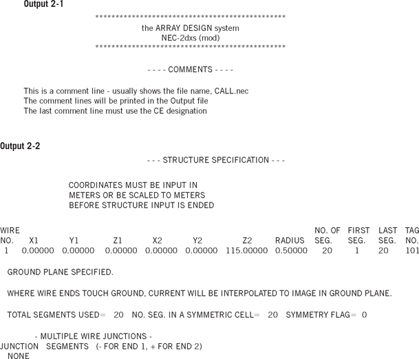
2.5.1 The Header
The header and comment lines are displayed at the start of the output file. See Output 2-1.
2.5.2 Structure Specifications
The wire geometry commands are listed under the heading — STRUCTURE SPECIFICATION —, as shown in Output 2-2.
Only one wire has been used in this example. Had additional wires been used, they would have been shown as additional printed lines in the output file and would be numbered under the heading WIRE NO.. For verification purposes, the X1, Y1, and Z1 headings show the coordinates of wire end 1. The coordinates of wire end 2 are X2, Y2, and Z2 and the wire radius is listed. The number of segments on the wire is shown, as well as the identifying numbers for those segments and the associated wire tag number.
The presence of a ground plane is verified, as is the ground image. A table of multiple-wire junctions listing any junctions at which three or more wires join is shown next, although this example has none. When multiple-wire junctions are present, the number of each segment connecting to the junction are printed, as a positive number if the reference direction of the segment is into the junction or a negative number if the reference direction is out of the junction.
2.5.3 Segmentation Data
Segment data is printed as shown in Output 2-3 (see page 20) under the heading- SEGMENTATION DATA — together with the angles ALPHA and BETA.
The angle Alpha is the vertical angle of the wire segment relative to the horizon. Zero degrees is horizontal and 90° is vertical. The angle alpha is used when calculating current moments in later chapters. Beta is the azimuth angle the wire makes relative to the coordinate system and is not currently used in any of the referenced postprocessing programs.
Within the subheading CONNECTION DATA the numbers under I—and I+ indicate the conditions at the first and second ends of segment number I, respectively. Segments connected at a junction can be located by tracing connection numbers through the table. After the sign is dropped, the connection number under I— or I+ is the number of the segment connecting to the end of segment I. If the sign of the connection number is positive, the segment reference directions are aligned (end 1 to end 2 or vice versa); if the number is negative, the reference directions are opposed (end 1 to end 1 or end 2 to end 2). When more than one segment connects to a segment end, the connection number gives the next connected segment in the sequence of segments, searching cyclically through the list.
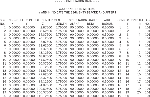
At a free end where the segment ends connects to nothing, the connection number is equal to zero.
One way of viewing the connection data is to recognize that the middle column is the segment of interest. To its right (I+) is the number of the next segment to which it connects. To its left (I—) is the number of the previous segment to which it is connected.
For example, notice the first entry, it is segment 1. To the right, it connects to segment 2. To its left, it connects to itself (segment 1) because the tower in this example is mounted over a perfectly conducting ground plane. Thus, the tower is connected to an image of itself in the ground.
Look now at the last entry in Output 2-3. It is segment 20. To the left of 20 is 19, which shows that the previous segment is 19. To the right is a zero, so segment 20 is open at that end.
Although it is not used very much in broadcast work, the utility of this listing will be more apparent when a more complex structure is displayed.
While the preceding may assist in confirming the correctness of the antenna geometry, there are several public domain programs available that will graphically display the antenna model. The program NVCOMP. EXE is one of these and is included on the disk associated with this book. Its use is covered in more detail in Appendix C.
2.5.4 Data Commands, Frequency, Loading, and Environment Data
Output 2-4 shows that the program control commands are listed in the output file for verification; the frequency and wavelength are stated;
Output 2-4
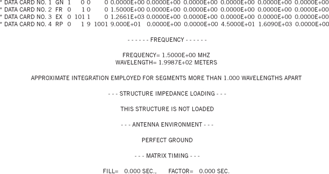

and if any segments had been impedance loaded (as is covered in Chapter 5), the loading will be listed for verification. The ground conditions are also shown together with some timing information.
2.5.5 Antenna Input Parameters
The data in Output 2-5 is very important to the broadcaster because it shows the drive point impedance of the antenna elements plus the power to each element. If more than one voltage source is used (as is the case in a directional array), each voltage source is shown as a separate line under the heading — ANTENNA INPUT PARAMETERS —. It is very important to remember that NEC-2 always works with PEAK values, not RMS. Both voltage and current values are peak values when read in the output file and also when specified in the input file.
The voltage listing is the voltage at the feed point of that tower. The power shown on a particular line is the power to that particular tower. In this example, the base voltage is shown as 1266.1 + j0.0 volts peak, the base current is 1.5797 + j3.6541 amp peak, the drive point impedance is 126.20 — j291.93, and the power into the tower is 1000 watts.
2.5.6 Currents and Location
Output 2-6 shows the data under the heading — CURRENTS AND LOCATIONS —, which include the coordinates and length of each segment and the current in that segment. From these listings, the current distribution on the tower can be determined and the current moments for each tower will be calculated. These listings are also used to determine the indications to be expected on the antenna monitor when the array is correctly adjusted. They are also used to determine the correct height on the tower at which to mount the antenna monitor's sample
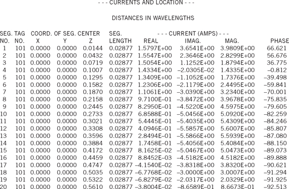
loop so that the antenna monitor will give indications closely representative of the corresponding far-field ratio.
It is important to recognize that the distances shown in this listing is given in units of wavelengths. This is done to make it easier for the reader to confirm that the segment lengths are reasonable. The segment lengths in meters can be found under the SEGMENTATION DATA heading or they can be easily calculated. In this example, the segments are all of the same length and are shown as 0.02877 λ, where λ is given under the FREQUENCY heading as 199.87 meters. Each segment is then 0.02877 × 199.87 = 5.75 meters.
2.5.7 Current Moments
An interesting aside here is to take a cursory (and perhaps oversimplified) look at the definition of a current moment as the term is used in this book. In mechanics, by definition a moment is the product of a quantity times a distance. A familiar moment in mechanics is torque, which is the product of a force, perhaps measured in pounds, times a distance, perhaps measured in feet. In that instance, the units of the moment torque would be foot-pounds. In a similar but simplified manner, a current moment is the product of a current, perhaps measured in amperes, and the distance over which that current flows, perhaps measured in meters. The units of current moment then are ampere-meters.
As shown in Output 2-6, the current flowing in each segment appears under the — CURRENT AND LOCATION — heading in the output file. Real/Imaginary notation is shown as well as the Magnitude/Phase. The length of each segment is also shown so the current moment can be calculated. For example, the current moment of segment 1 is (1.5797 + j3.6541)5.75 = 9.08 + j21.01, or 22.89 @ 66.62° amp-meters. In a similar manner, the current moment of segment 20 is calculated to be only −0.22 – j4.98, or 4.98 @ −92.51° amp-meters.
The total current moment of the tower is the vector sum of the individual current moments of all 20 segments.
2.5.8 Power Budget
The input power, shown under the heading — POWER BUDGET — in Output 2-7 is the total power, summed from all towers and losses of the system. No losses have been included in this simple example so the efficiency is 100 percent. The radiated power is the input power less the power losses.
2.5.9 Radiation Pattern
The listings under — RADIATION PATTERNS — in Output 2-8 show the vertical angle, theta, at which the pattern is calculated versus the azimuth angle, phi.
These angles are explained in more detail in the Geometry section but it is necessary to explain now that the vertical angle, Theta, is
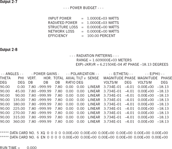
measured from the zenith overhead as 0°, making the horizon 90°. Thus a horizontal pattern is calculated with a value of theta = 90°, not 0° The field shown as E(THETA) is the vertically polarized component of radiation and E(PHI) is the horizontally polarized component.
Because the radiation is from a single vertical tower, the horizontally polarized component, E(PHI), is zero and the magnitude of the vertically polarized component, E(THETA), is the same at all azimuth angles, phi.
2.6 Exercises
2-1. Do a bnec.exe run using the example code given in Section 2.4.4, Listing 2-1 as the input file and record the drive point impedance.
2-2. The example code given in Section 2.4.4 as Listing 2-1 specifies a drive voltage of 1266.084 volts at 0°. Modify the Listing 2-1 code to specify the drive voltage as 1266.084 volts at an angle of 60°. Do a bnec.exe run using the modified code as the input file and compare the modified code drive point impedance with the original drive point impedance obtained in exercise 2–1. Explain the comparison.
2-3. Using the data given in the output file created by the modified listing in exercise 2–2, calculate the total current moment for the tower. How does this current moment compare with that determined from the output data of exercise 2-1? Why?