
Chapter 2
Audio Basics
This chapter covers the following topics:
Basic Understanding of Sound: This topic will introduce a basic understanding of how sound behaves, including wave propagation, technical properties of sound waves, and noise.
Analog vs. Digital Signals: This topic will compare noise on an analog signal compared to noise on a digital signal, observe the principle of the Nyquist-Shannon theorem, and identify how bandwidth conservation can be achieved through data compression.
ITU Audio Encoding Formats: This topic will identify the most commonly used audio codecs in a Cisco solution and analyze the various aspects of each codec.
The preceding chapter provided a backward look into the evolution of communications and a high-level overview of the technologies that exist today that allow us to collaborate at many levels. This chapter will begin to dive into the intricate details that encompass the vast world of audio communication. As you read through this chapter, you will find that the chasm that embodies audio communication is only a foot wide but a mile deep. Although this chapter will not cover every aspect of audio communication, it will provide a solid foundation to build your knowledge on. Topics discussed in this chapter include the following:
Basic Understanding of Sound
Wave Propagation
Technical Properties of a Sound Wave
Understanding Noise
Analog vs. Digital Signals
Nyquist-Shannon Sampling Theorem
Data Compression Equals Bandwidth Conservation
ITU Audio Encoding Formats
This chapter covers the following objective from the Cisco Collaboration Core Technologies v1.0 (CLCOR 350-801) exam:
2.2 Identify the appropriate collaboration codecs for a given scenario
“Do I Know This Already?” Quiz
The “Do I Know This Already?” quiz allows you to assess whether you should read this entire chapter thoroughly or jump to the “Exam Preparation Tasks” section. If you are in doubt about your answers to these questions or your own assessment of your knowledge of the topics, read the entire chapter. Table 2-1 lists the major headings in this chapter and their corresponding “Do I Know This Already?” quiz questions. You can find the answers in Appendix A, “Answers to the ‘Do I Know This Already?’ Quizzes.”
Table 2-1 “Do I Know This Already?” Section-to-Question Mapping
Foundation Topics Section |
Questions |
|---|---|
Basic Understanding of Sound |
1–4 |
Analog vs. Digital |
5–8 |
ITU Audio Encoding Formats |
9–10 |
Caution
The goal of self-assessment is to gauge your mastery of the topics in this chapter. If you do not know the answer to a question or are only partially sure of the answer, you should mark that question as wrong for purposes of the self-assessment. Giving yourself credit for an answer you correctly guess skews your self-assessment results and might provide you with a false sense of security.
1. Through which of the following mediums will sound travel the fastest?
Air
Water
Concrete
Gypsum board
2. The measure of the magnitude of change in each oscillation of a sound wave is a description of which term?
Frequency
Amplitude
Wavelength
Pressure
3. Which of the following is used to calculate the average amplitude of a wave over time?
Newton’s second law of motion
Sine waves
Pascals
Root mean squared
4. What is the primary issue with using repeaters for analog signals?
Noise riding on the original audio signal is also amplified by the repeaters.
Distances may be too great to host enough repeaters.
Noise from the repeaters can be interjected into the audio signals.
There are no issues with using a repeater for analog signals.
5. Which of the following is a benefit of digital audio over analog audio?
Digital signals are more fluid than analog signals.
Digital signals have a more natural sound than analog signals.
Digital signals are immune to ambient noise.
Digital signals are not based on timing like an analog signal is.
6. What is the maximum bit rate the human ear can hear at?
24 bit
21 bit
144 bit
124 bit
7. Which of the following supports 24 circuit channels at 64 Kbps each?
DS0
DS1
T3
E1
8. Which of the following describes lossless compression?
This algorithm searches content for statistically redundant information that can be represented in a compressed state.
This algorithm searches for nonessential content that can be deleted to conserve storage space.
Compression formats suffer from generation loss.
Repeatedly compressing and decompressing the file will cause it to progressively lose quality.
9. Which of the following codecs supports both compressed and uncompressed data?
G.711
G.729
G.722
G.723.1
10. Which of the following codecs supports lossless compression?
G.729
G.722
iLBC
iSAC
Foundation Topics
Basic Understanding of Sound
Sound is the traveling of vibrations through a medium, which in most cases is air, generated by a source as waves of changing pressure. These waves of changing pressure in the air, in turn, vibrate our eardrums, allowing our brains to perceive them as sound. How often these pulses of pressure change in a given time period can be measured. We can also measure how intense each pressure change is and how long the space is between each wave. Two factors that relate to sound must be considered: the source and the medium.
Anything that can create these vibrations can be the source of sound. These sources could include human vocal cords or animal larynx, such as birds chirping, lions roaring, or dogs barking. Sound could also be sourced from stringed instruments, such as a guitar, violin, or cello. Percussions cause sound, such as drum skins or even the diaphragm of a loudspeaker. All these things in some way vibrate particles to make sound. A tree falling in the forest will make sound, whether you hear it or not.
The medium sound travels through can affect how that sound is perceived. Have you ever dipped your head underwater in a swimming pool and tried to talk with someone else? Although you can hear the other person, understanding what that person is saying becomes difficult, even when you are both in close proximity. It’s important to understand that the speed of sound is constant within a given medium at a given temperature. Generally, the term speed of sound refers to a clear, dry day at about 20° C (68° F), which would have the speed of sound at 343.2 meters per second (1,126 ft/s). This equates to 1,236 kilometers per hour (768 mph)—about 1 kilometer in 3 seconds or approximately 1 mile in 5 seconds. The denser the medium, the faster sound will travel. Because air is thicker at lower elevations, and temperatures are usually higher, sound will travel faster but will degrade faster as well. However, in a vacuum, sound will travel much slower because there are no particles to propagate the sound waves, but sound can be heard much clearer at farther distances because they will degrade much slower. Table 2-2 illustrates the speed of sound through four different mediums.
Table 2-2 Speed of Sound Through Four Common Mediums
Medium |
Speed (Meters per Second) |
Speed (Feet per Second) |
Speed Factor |
|---|---|---|---|
Air |
344 |
1130 |
1 |
Water |
1480 |
4854 |
4.3 |
Concrete |
3400 |
11,152 |
9.8 |
Gypsum Board |
6600 |
22,305 |
19.6 |
Wave Propagation
Stand next to a still body of water, pick up a pebble, and toss it to the middle of the pond. As the pebble breaks the surface, it displaces the water it comes in immediate contact with. Those water particles displace other water particles as they are pushed out, so you get a rippling effect that grows from the point where the pebble originally made contact out to the edges of the pond. Once the ripples meet the outer edges of the pond, the rings will begin to move back in, and the ripples will continue until the energy created by tossing the pebble into the water runs out.
This principle is the same one on which sound propagates. When sound is created at the source, the vibrations radiate out in waves, like the ripples in a pond, except they travel in every direction. These sound waves bounce off particles of different mediums in order to travel outward. As the sound waves bounce off particles, some of the energy is absorbed so the vibration weakens. The density of a medium plays a part in how fast a sound wave can propagate or move through it. The more tightly that particles of matter are packed together, the faster a sound wave will move through it, but the sound wave will degrade faster as well. So sound travels faster through a solid than a liquid and faster through a liquid than a gas, such as air. As the sound expands across a larger area, the power that was present at the source to create the original compression is dissipated. Thus, the sound becomes less intense as it progresses farther from the source. The sound wave will eventually stop when all the energy present in the wave has been used up moving particles along its path.
Observe the analogy of the pebble in the pond. When the ripples first begin, they will be taller and closer together. As the energy dissipates, the ripples will become shorter and farther apart, until eventually they cease to demonstrate any effect on the water’s surface. This effect can be observed with sound as well. Stand in a canyon and shout out toward the cliffs. The sound you create will travel out and reverberate off the cliffs and return to you. However, what you hear will sound degraded. You may even hear yourself multiple times in an echo, but each time the sound will be weaker than the time before until you can’t hear anything at all. If someone shouted out to you under a body of water, by the time the sound reached your ears, it would have degraded so much from bouncing off all the many particles in the water that you would not be able to articulate what was said.
Technical Properties of Sound
All forms of energy can be measured. Light and sound sources in nature are forms of energy. Acoustical energy consists of fluctuating waves of pressure, generally in the air. One complete cycle of that wave consists of a high- and low-pressure half-cycle. This means that half of a sound wave is made up of the compression of the medium, and the other half is the decompression, or rarefaction, of the medium. Imagine compressing a spring and then letting it go. Now imagine that the spring represents air molecules and your hand is the acoustic energy. Figure 2-1 illustrates the technical properties of a sound wave.

Figure 2-1 Technical Properties of a Sound Wave
To better understand how sound waves are measured, we must define some terms. Frequency is the rate of the air pressure fluctuation produced by the acoustic energy wave. To be heard by human ears, wave frequencies must be between 20 and 20,000 cycles per second. Although there is more to it than just frequency, in general, the frequency of a sound wave corresponds with the perceived pitch of the sound. The higher the pitch, the higher the frequency. When we are talking about sounds and music, there is not just one single frequency, but many different frequencies overlapping with each other. This means many different frequencies are being represented within a single signal. The bandwidth of a particular signal is the difference between the highest and the lowest frequencies within the signal.
Amplitude is the measure of the magnitude of change in each oscillation of a sound wave. Most often this measurement is peak-to-peak, such as the change between the highest peak amplitude value and the lowest trough amplitude value, which can be negative. Bear in mind the relationship between amplitude and frequency. Two waveforms can have identical frequency with differing amplitude and identical amplitude with differing frequency. For sound waves, the wave oscillations are representative of air molecules moving due to atmospheric pressure changes, so the amplitude of a sound wave is a measure of sound pressure. Sound pressure is measured in pascals or millibars:
1 pascal = 1 newton per square meter
1 millibar = 100 pascals
A newton is the standard international unit for force. It is equal to the amount of net force required to accelerate a mass of one kilogram at a rate of one meter per second squared. Newton’s second law of motion states F = ma, multiplying m (kg) by a (m/s2); the newton is, therefore, N = kg(m/s2).
A frequency spectrum is the complete range of frequencies that can be heard, just as the visible spectrum is the range of light frequencies that can be seen. Devices and equipment can also have frequency spectrums, or ranges.
Basic sine waves cannot have an “average” per se. Rather, it would equal zero because the wave peaks and valleys are symmetrical above and below the reference of zero. What is much more helpful when discussing the average amplitude of a wave over time is called root mean squared (RMS). RMS is often used to calculate a comparable measure of power efficiency, such as in audio amplifiers. RMS measures mean output power to mean input power. RMS is just the squaring of every point of a wave and then finding the average. Squaring a negative value always results in a positive value. RMS gives us a useful average value for discussing audio equipment and comparing amplitude measurements. Basically, RMS is much more similar to the way we hear sound, as opposed to measuring just the peaks of a wave, because we don’t hear just the peaks.
A sound wave emanating from a source is like an expanding bubble. The power of the sound would be the energy on the surface of the bubble. As the surface of the bubble expands, that energy is used up in order to move, or vibrate, the air ever farther outward. That means eventually the power that the bubble started with at its source would be expended. The power of sound, or sound’s acoustical power, is a measure of amplitude over time. The sound had a particular measurement at the moment it was emitted from the source, but as it travels, over time the power decreases as the energy present in the sound wave is expended transmitting itself through the medium. The transmission of acoustical energy through a medium is measured in watts. A watt is just the rate of transfer of energy in one second or one joule per second. A joule is equal to the energy expended in applying a force of one newton through a distance of one meter. The following equation is used to calculate sound’s acoustical power:
J=kg*m2/s2=N*4444m=Pa*m3=W*s
where
N is the newton.
m is the meter.
kg is the kilogram.
s is the second.
Pa is the pascal.
W is the watt.
Understanding Attenuation and Noise
When Alexander Graham Bell placed his first audio call to his assistant, Watson, it was only to the next room. Bell’s journal records that the audio was loud but muffled. There are two reasons why the sound was hard to hear: attenuation and noise.
Attenuation, as has previously been discussed, is the degrading of the sound wave as it loses energy over time and space. When the telephone was first made available to the public market, telephone companies had to set up repeaters to account for this loss in signal strength. These repeaters could boost the intensity of the analog wave at different points along the path between two telephones, or nodes. This allowed telephone calls to traverse much longer distances. However, telephone repeaters solved only half the problem.
In audio terms, noise doesn’t necessarily refer to something you hear. Noise can also refer to inaccuracies or imperfections in a signal transmission that was not intended to be present. Noise comes in different forms, like acoustical, digital, or electrical. Noise can be introduced to a signal in many ways, like faulty connections in wiring or external signal interference. In telephony, as audio signals are transmitted across a wire using electrical signals, those same wires can pick up energy from external sources and transmit them along the same current carrying the audio signal. If you are old enough to remember using analog phones, you might also remember hearing a crackling sound in the background during a phone call. That background noise was caused by interference.
When an analog signal must be transmitted a long distance, the signal level is amplified to strengthen it; however, this process also amplifies any noise present in the signal. This amplification could cause the original analog signal to become too distorted to be heard properly at the destination. Therefore, it is very important with analog transmissions to make sure the original audio signal is much stronger than the noise. Electronic filters can also be introduced, which helps remove unwanted frequency from the analog signal. The frequency response may be tailored to eliminate unwanted frequency components from an input signal or to limit an amplifier to signals within a particular band of frequencies. Figure 2-2 illustrates how noise riding on an analog signal can be amplified at repeaters.
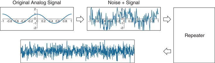
Figure 2-2 Amplification of Noise on an Analog Signal
Analog vs. Digital Signals
An analog signal is a continuous signal that contains a time variable representative of some other time-varying quality, such as the voltage of the signal may vary with the pressure of the sound waves. In contrast, a digital signal is a continuous quantity that is a representation of a sequence of discrete values which can take on only one of a finite number of values. There are only two states to a digital bit, zero or one, which can also be perceived as on or off. These are referred to as binary digits. Another way to compare analog signals with digital signals could be to think of them as light switches. A digital signal operates like a regular light switch; it is either on or off. An analog signal is more like a dimmer switch that is fluid and allows varying levels of light.
Another good way to mentally picture the difference between analog and digital is to think of two types of clocks. An analog clock has hands that point at numbers, by slowly rotating around in a circle, and digital clocks have decimal number displays. The analog clock has no physical limit to how finely it can display the time, as its hands move in a smooth, pauseless fashion. If you look at the clock at just the right moments, you can see the hand pointing between two minutes or even two seconds, such as it could read 3:05 and a half. The digital clock cannot display anything between 3:05 and 3:06. It is either one or the other; there is no variance between the two times.
When it comes to sound quality, there is much debate as to whether analog or digital sounds better. Vinyl records, or LP (long play) records, are an example of raw analog audio that has been recorded. CDs or MP3s are examples of digital audio that has been recorded. The science behind audio quality definitively determines that analog has a better sound quality than digital because analog is the most natural and raw form of sound waves, and analog is the only form of audio sound waves our ears can articulate. Digital recordings take an analog signal and convert it into a digital format. When that digital recording is played back, it must be converted back to analog before the audio is played over speakers. Because digital conversion cannot make a perfect copy of the original fluid audio sound wave, some of that sound quality is lost when the digital signal is converted back into analog.
This issue of conversion raises a question: if analog audio is better than digital audio, why use digital at all? In conjunction with the preceding examples, digital copies allow a higher quantity of audio to be stored. If you go to a music store or download music from the Internet, you can store more songs in a smaller container, such as an MP3 player or an iPod. Bringing the subject back to communications, an analog signal cannot travel very far without suffering from attenuation. Digital signals can travel much farther than analog signals and don’t degrade in the same manner. Digital repeaters will amplify the signal, but they may also retime, resynchronize, and reshape the pulses. Additionally, analog signals are very sensitive to ambient noise, which can quickly degrade the sound quality. Digital signals use binary digits of zero or one, so they are immune to ambient noise.
It is much easier to identify and remove unwanted noise from a digitally sampled signal compared to an analog signal. The intended state of the signal is much easier to recognize. When discussing potential errors in a transmitted signal, error checking and correction are made much easier by the very nature of digital representation. As a digital signal enters a digital repeater, an algorithm will first check to see if the information that is supposed to be there still exists or if it’s missing. Assuming the correct information is there, next it will check the state of each digital bit in question: on or off (a one or zero). Finally, it will check that the position of each bit is correct: is the bit on when it’s supposed to be off or vice versa?
When an analog signal must be transmitted a long distance, the signal level is amplified to strengthen it; however, this also amplifies any noise present in the signal. Digital signals are not amplified. Instead, for long-distance transmission, the signal is regenerated at specific intervals. In this manner, noise is not passed along the transmission chain.
Nyquist-Shannon Sampling Theorem
Always keep in mind that digital signals are just long strings of binary numbers. Analog signals must be somehow converted into strings of numbers to be transmitted in the digital realm. When a continuous analog signal is converted to a digital signal, measurements of the analog signal must be taken at precise points. These measurements are referred to as samples. The more frequent the sample intervals, the more accurate the digital representation of the original analog signal. The act of sampling an analog signal for the purpose of reducing it to a smaller set of manageable digital values is referred to as quantizing or quantization. The difference between the resulting digital representation of the original analog signal and the actual value of the original analog signal is referred to as quantization error. Figure 2-3 illustrates how quantizing an analog signal would appear.

Figure 2-3 Quantizing an Analog Signal
In Figure 2-3, each movement upward on the Y-axis is signified by a one-binary digit. Each movement horizontally on the X-axis is signified by a zero-binary digit. Each movement downward on the Y-axis is signified by a negative one-binary digit. In this manner an analog signal can be quantized into a digital signal. However, notice that the binary signal is not exactly the same as the original analog signal. Therefore, when the digital signal is converted back to analog, the sound quality will not be the same. A closer match can be obtained with more samples. The size of each sample is measured in bits per sample and is generally referred to as bit depth. However, it will never be exact because a digital signal cannot ever match the fluid flow of an analog signal. The question becomes, can a digital signal come close enough to an analog signal that it is indistinguishable to the human ear?
When an audio signal has two channels, one for left speakers and one for right speakers, this is referred to as stereo. When an audio signal has only one channel used for both left and right speakers, this is referred to as mono. Using the preceding quantizing information, along with whether an audio signal is stereo or mono, it is relatively simple to calculate the bit rate of any audio source. The bit rate describes the amount of data, or bits, transmitted per second. A standard audio CD is said to have a data rate of 44.1 kHz/16, meaning that the audio data was sampled 44,100 times per second, with a bit depth of 16. CD tracks are usually stereo, using a left and right track, so the amount of audio data per second is double that of mono, where only a single track is used. The bit rate is then 44,100 samples/second × 16 bits/sample × 2 tracks = 1,411,200 bps or 1.4 Mbps.
When the sampling bit depth is increased, quantization noise is reduced so that the signal-to-noise ratio, or SNR, is improved. The relationship between bit depth and SNR is for each 1-bit increase in bit depth, the SNR will increase by 6 dB. Thus, 24-bit digital audio has a theoretical maximum SNR of 144 dB, compared to 96 dB for 16-bit; however, as of 2007 digital audio converter technology is limited to an SNR of about 126 dB (21-bit) because of real-world limitations in integrated circuit design. Still, this approximately matches the performance of the human ear. After about 132 dB (22-bit), you would have exceeded the capabilities of human hearing.
To determine the proper sampling rate that must occur for analog-to-digital conversion to match the audio patterns closely, Harry Nyquist and Claude Shannon came up with a theorem that would accurately calculate what the sampling rate should be. Many audio codecs used today follow the Nyquist-Shannon theorem. Any analog signal consists of components at various frequencies. The simplest case is the sine wave, in which all the signal energy is concentrated at one frequency. In practice, analog signals usually have complex waveforms, with components at many frequencies. The highest frequency component in an analog signal determines the bandwidth of that signal. The higher the frequency, the greater the bandwidth, if all other factors are held constant. The Nyquist-Shannon theorem states that to allow an analog signal to be completely represented in digital form, the sampling rate must be at least twice the maximum cycles per second, based on frequency or bandwidth, of the original signal. This maximum bandwidth is called the Nyquist frequency. If the sampling rate is not at least twice the maximum cycles per second, then when such a digital signal is converted back to analog form by a digital-to-analog converter, false frequency components appear that were not in the original analog signal. This undesirable condition is a form of distortion called aliasing. Sampling an analog input signal at a rate much higher than the minimum frequency required by the Nyquist-Shannon theorem is called over-sampling. Over-sampling improves the quality or the digital representation of the original analog input signal. Under-sampling occurs when the sampling rate is lower than the analog input frequency.
The Nyquist-Shannon theorem led to the Digital Signal 0 (DS0) rate. DS0 was introduced to carry a single digitized voice call. For a typical phone call, the audio sound is digitized at an 8 kHz sample rate using 8-bit pulse-code modulation for each of the 8000 samples per second. This resulted in a data rate of 64 kbps.
Because of its fundamental role in carrying a single phone call, the DS0 rate forms the basis for the digital multiplex transmission hierarchy in telecommunications systems used in North America. To limit the number of wires required between two destinations that need to host multiple calls simultaneously, a system was built in which multiple DS0s are multiplexed together on higher-capacity circuits. In this system, 24 DS0s are multiplexed into a DS1 signal. Twenty-eight DS1s are multiplexed into a DS3. When carried over copper wire, this is the well-known T-carrier system, with T1 and T3 corresponding to DS1 and DS3, respectively.
Outside of North America, other ISDN carriers use a similar Primary Rate Interface (PRI). Japan uses a J1, which essentially uses the same 24 channels as a T1. Most of the world uses an E1, which uses 32 channels at 64 kbps each. ISDN will be covered in more depth in Chapter 5, “Communication Protocols.” However, it is important to note that the same sampling rate used with DS0 is also used in VoIP communications across the Internet. This led to a new issue that in turn opened up a new wave of advancement in the audio communication industry: How could digital audio signals be sent over low-bandwidth networks?
Data Compression Equals Bandwidth Conversion
The answer to the question regarding digital audio signals being sent over low-bandwidth networks came with the development of data compression. Bandwidth is the rate that data bits can successfully travel across a communication path. Transmitting audio can consume a high amount of bandwidth from a finite total available. The higher the sampled frequency of a signal, the larger the amount of data to transmit, resulting in more bandwidth being required to transmit that signal. Data compression can reduce the amount of bandwidth consumed from the total transmission capacity. Compression involves utilizing encoding algorithms to reduce the size of digital data. Compressed data must be decompressed to be used. This extra processing imposes computational or other costs into the transmission hardware.
Lossless and lossy are descriptive terms used to describe whether or not the data in question can be recovered exactly bit-for-bit when the file is uncompressed or whether the data will be reduced by permanently altering or eliminating certain bits, especially redundant bits. Lossless compression searches content for statistically redundant information that can be represented in a compressed state without losing any original information. By contrast, lossy compression searches for nonessential content that can be deleted to conserve storage space. A good example of lossy would be a scenic photo of a house with a blue sky overhead. The actual color of the sky isn’t just one color of blue; there are variances throughout. Lossy compression could replace all the blue variances of the sky with one color of blue, thus reducing the amount of color information needed to replicate the blue sky after decompression. This is, of course, an unsubtle oversimplification of the process, but the concept is the same.
It is worth noting that lossy compression formats suffer from generation loss; repeatedly compressing and decompressing the file will cause it to progressively lose quality. This is in contrast with lossless data compression, where data will not be lost even if compression is repeated numerous times. Lossless compression therefore has a lower limit. A certain amount of data must be maintained for proper replication after decompression. Lossy compression assumes that there is a trade-off between quality and the size of the data after compression. The amount of compression is limited only by the perceptible loss of quality that is deemed acceptable.
ITU Audio Encoding Formats
Codec stands for coding and decoding. A codec is a device or software program that is designed to code and decode digital data, as well as compress and decompress that data. Therefore, an audio codec is a device or software that is designed to process incoming analog audio, convert it to digital, and compress the data, if necessary, before sending that data to a specific destination. The codec can also process incoming data, decompress that data if necessary, and convert the digital data back to analog audio. Many proprietary codecs have been created over the years. However, in an effort to unify communications, the International Telecommunications Union (ITU) created a standardized set of audio codecs. The ITU is a specific agency of the United Nations whose chief responsibilities include the coordination of the shared global use of the usable RF spectrum, and the establishment of standards to which manufacturers and software designers comply in order to ensure compatibility. Table 2-3 outlines some of the more common audio codecs used in a Cisco collaboration solution. Each codec that starts with a “G” is an ITU codec.
Table 2-3 Audio Codecs Commonly Used by Cisco
Codec and Bit Rate (Kbps) |
Codec Sample Size (Bytes) |
Codec Sample Interval (ms) |
Mean Opinion Score (MOS) |
Voice Payload Size (Bytes) |
Bandwidth MP or FRF.12 (Kbps) |
Bandwidth Ethernet (Kbps) |
|---|---|---|---|---|---|---|
G.711 (64 Kbps) |
80 |
10 |
4.1 |
160 |
82.8 |
87.2 |
G.729 (8 Kbps) |
10 |
10 |
3.92 |
20 |
26.8 |
31.2 |
G.723.1 (6.3 Kbps) |
24 |
30 |
3.9 |
24 |
18.9 |
21.9 |
G.723.1 (5.3 Kbps) |
20 |
30 |
3.8 |
20 |
17.9 |
20.8 |
G.726 (32 Kbps) |
20 |
5 |
3.85 |
80 |
50.8 |
55.2 |
G.726 (24 Kbps) |
15 |
5 |
60 |
42.8 |
47.2 |
|
G.728 (16 Kbps) |
10 |
5 |
3.61 |
60 |
28.5 |
31.5 |
G.722_64k (64 Kbps) |
80 |
10 |
4.13 |
160 |
82.8 |
87.2 |
iLBC_Mode_20 (15.2 Kbps) |
38 |
20 |
4.14 |
38 |
34.0 |
38.4 |
iLBC_Mode_30 (13.33 Kbps) |
50 |
30 |
4.14 |
50 |
25.867 |
28.8 |
Table 2-3 is not an exhaustive list of codecs available today, and it is important to note that ITU codecs are used with SIP communication as well. Table 2-3 is divided into seven columns. The first column identifies the codec and the number of bits per second needed to transmit the payload in each packet for a voice call. The codec bit rate = codec sample size / codec sample interval. The next column is the codec sampling size based on bytes. This is the number of bytes captured by the codec at each codec sample interval. Column three is the codec sampling interval. This is the sample interval at which the codec operates. For example, the G.729 codec operates on sample intervals of 10 ms, corresponding to 10 bytes (80 bits) per sample at a bit rate of 8 kbps. The next column is the Mean Opinion Score (MOS), which is a system of grading the voice quality of telephone connections. With MOS, a wide range of listeners judge the quality of a voice sample on a scale of one (bad) to five (excellent). The scores are averaged to provide the MOS for the codec. The last two columns show the bandwidth needed to transmit the audio with overhead added in. The bandwidth MP or FRF.12 shows the Layer 2 header values added to the original payload, and the bandwidth ethernet shows the Layer 3 header values added on top of the Layer 2 headers.
Based on the Nyquist-Shannon theorem, the first audio codec created by the ITU is G.711. Originally released in 1972, G.711 is also referred to as pulse-code modulation (PCM) and was introduced for use in telephony. It is the required minimum standard in both H.320 for circuit-switched telephony and H.323 for packet-switched telephony. It is considered a narrow-band codec since it processes only frequencies between 300 and 3400 Hz, although an annex has been added to extend the frequency range. It uses a sampling frequency of 8 kHz and has a bit rate of 64 kbps. Two algorithm types are associated with G.711: G.711 mu-law and G.711 a-law. G.711 mu-law is a companding algorithm, which reduces the dynamic range of an audio signal. G.711 mu-law is used throughout North America and Japan. The algorithm used with G.711 a-law is common throughout the rest of the world where E1 circuits are used, and it is the inverse of the mu-law algorithm. All G.711 codecs are uncompressed.
G.729 is a lossy compressed audio codec and is the most common compression algorithm used in low-bandwidth environments. It has been used in videoconferencing applications for some time and attained its ITU recommendation in 1996. It can operate at a low rate of 4000 Hz. There are several annexes to the G.729 codec, the ones most commonly used with Cisco being G.729r8 and G.729br8. Both codecs operate at 8 Kbps, but G.729br8 contains built-in VAD that cannot be disabled.
Now compare the two previously mentioned codecs with G.722. Released in 1988, this codec can operate as a lossy compressed codec or an uncompressed codec, depending on the annex being run. G.722 addressed some of the speech quality issues presented by the limited bandwidth of the G.711 codec. In contrast to G.711, G.722 is considered a wide-band codec and processes frequencies between 50 and 7000 Hz. It also samples audio at 16 kHz and operates at 48, 56, or 64 kbps. When G.722 audio is used over an H.323 call, the packets are framed using the 802.3 standard and are sent at 60-millisecond intervals.
Two other commonly used codecs with Cisco collaboration solutions are iLBC and iSAC. These are not ITU codecs, but they are open standards that can be used by any organization. Internet Low Bitrate Codec (iLBC) was originally drafted for the WebRTC project. It was adopted by the IETF in 2002 and ratified into SIP communications in 2003. Internet Speech Audio Codec (iSAC) was originally created by Global IP Solutions. iSAC was acquired by Google in 2011, incorporated into the open-source WebRTC project, and later ratified into the SIP protocol by the IETF. The iSAC codec is an adaptive wideband speech and audio codec that operates with short delay, making it suitable for high-quality real-time communication. It is specially designed to deliver wideband speech quality in both low and medium bit-rate applications. The iSAC codec compresses speech frames of 16 kHz, 16-bit sampled input speech, each frame containing 30 or 60 ms of speech. The codec runs in one of two different modes called channel-adaptive mode and channel-independent mode. In both modes iSAC is aiming at a target bit rate, which is neither the average nor the maximum bit rate that will be reached by iSAC, but it corresponds to the average bit rate during peaks in speech activity.
In channel-adaptive mode, the target bit rate is adapted to give a bit rate corresponding to the available bandwidth on the channel. The available bandwidth is constantly estimated at the receiving iSAC and signaled in-band in the iSAC bit stream. Even at dial-up modem data rates, iSAC delivers high quality by automatically adjusting transmission rates to give the best possible listening experience over the available bandwidth. The default initial target bit rate is 20,000 bits per second in channel-adaptive mode.
In channel-independent mode, a target bit rate has to be provided to iSAC prior to encoding. After encoding the speech signal, the iSAC codec uses lossless coding to further reduce the size of each packet and hence the total bit rate used. The adaptation and the lossless coding described here both result in a variation of packet size, depending both on the nature of speech and the available bandwidth. Therefore, the iSAC codec operates at transmission rates from about 10 kbps to about 32 kbps.
The best quality audio codec available to date is Advanced Audio Codec-Low Delay (AAC-LD). It is also referred to as Low-overhead MPEG-4 Audio Transport Multiplex (LATM), and this codec is most commonly used with SIP communication. Since 1997 this codec has been used to offer premium stereo audio by over-sampling analog audio signaling. Sampling rates range between 48 Kbps and 128 Kbps, with a frequency range of 20 kHz. Although this codec does offer excellent audio quality during calls, the trade-off is the high cost in bandwidth when this codec is used.
Exam Preparation Tasks
As mentioned in the section “How to Use This Book” in the Introduction, you have a couple of choices for exam preparation: the exercises here, Chapter 32, “Final Preparation,” and the exam simulation questions in the Pearson Test Prep Software Online.
Review All Key Topics
Review the most important topics in this chapter, noted with the Key Topics icon in the outer margin of the page. Table 2-4 lists a reference of these key topics and the page numbers on which each is found.
Table 2-4 Key Topics for Chapter 2
Key Topic Element |
Description |
Page Number |
|---|---|---|
Speed of Sound Through Four Common Mediums |
19 |
|
Paragraph |
Behavior of Sound Waves as They Propagate |
19 |
Section |
Technical Properties of Sound |
20 |
Paragraph |
Define Attenuation and Noise |
22 |
Paragraph |
Define Analog and Digital Audio Signals |
23 |
Paragraph |
Samples and Quantization Explained |
24 |
Paragraph |
Nyquist-Shannon Theorem Explained |
25 |
Paragraph |
Lossless and Lossy Compression Explained |
26 |
Audio Codecs Commonly Used by Cisco |
27 |
|
Paragraph |
G.711, G.729, and G.722 Explained |
28 |
Define Key Terms
Define the following key terms from this chapter and check your answers in the glossary:
Q&A
The answers to these questions appear in Appendix A. For more practice with exam format questions, use the Pearson Test Prep Software Online.