Introduction

The systematic study of character sums over finite fields may be said to have begun over 200 years ago, with Gauss. The Gauss sums over F_p are the sums

for à a nontrivial additive character of F_p, e.g., x e^2πix/p, and χ a nontrivial multiplicative character of F^×_p. Each has absolute value √p. In 1926, Kloosterman [Kloos] introduced the sums (one for each a ∈ F^×_p)

which bear his name, in applying the circle method to the problem of four squares. In 1931 Davenport [Dav] became interested in (variants of) the following questions: for how many x in the interval [1, p – 2] are both x and x + 1 squares in F_p? Is the answer approximately p/4 as p grows? For how many x in [1, p – 3] are each of x, x + 1, x + 2 squares in F_p? Is the answer approximately p/8 as p grows? For a fixed integer r ≥ 2, and a (large) prime p, for how many x in [1, p – r] are each of x, x + 1, x + 2, …, x + r – 1 squares in F_p. Is the answer approximately p/2^r as p grows? These questions led him to the problem of giving good estimates for character sums over the prime field F_p of the form

where χ₂ is the quadratic character χ₂(x) := and where f(x) ∈ F_p[x] is a polynomial with all distinct roots. Such a sum is the “error term” in the approximation of the number of mod p solutions of the equation

y² = f(x)

by p, indeed the number of mod p solutions is exactly equal to

And, if one replaces the quadratic character by a character χ of F^×_p of higher order, say order n, then one is asking about the number of mod p solutions of the equation

yⁿ = f(x).

This number is exactly equal to

The “right” bounds for Kloosterman’s sums are

for a ∈ F^×_p. For f(x) = ∑^d_i=0 a_ixⁱ squarefree of degree d, the “right” bounds are

for χ nontrivial and χ^d ≠ , and

for χ nontrivial and χ^d = . These bounds were foreseen by Hasse [Ha-Rel] to follow from the Riemann Hypothesis for curves over finite fields, and were thus established by Weil [Weil] in 1948.

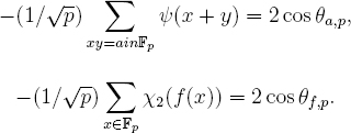
Following Weil’s work, it is natural to “normalize” such a sum by dividing it by √p, and then ask how it varies in an algebro-geometric family. For example, one might ask how the normalized¹ Kloosterman sums

vary with a ∈ F^×_p, or how the sums

vary as f runs over all squarefree cubic polynomials in F_p[x]. [In this second case, we are looking at the F_p-point count for the elliptic curve y² = f(x).] Both these sorts of normalized sums are real, and lie in the closed interval [–2, 2], so each can be written as twice the cosine of a unique angle in [0, π]. Thus we define angles θ_a,p, a ∈ F^×_p, and angles θ_f,p, f a squarefree cubic in F_p[x]:

In both these cases, the Sato-Tate conjecture asserted that, as p grows, the sets of angles {θ_a,p}_{a ∈ F^×p} (respectively {θ_f,p}_{f ∈ Fp[x] squarefree cubic}) become equidistributed in [0, π] for the measure (2/π)sin²(θ)dθ. Equivalently, the normalized sums themselves become equidistributed in [–2, 2] for the “semicircle measure” (1/2π)√4 – x²dx. These Sato-Tate conjectures were shown by Deligne to fall under the umbrella of his general equidistribution theorem, cf. [De-Weil II, 3.5.3 and 3.5.7] and [Ka-GKM, 3.6 and 13.6]. Thus for example one has, for a fixed nontrivial χ, and a fixed integer d ≥ 3 such that χ^d ≠ , a good understanding of the equidistribution properties of the sums

as f ranges over various algebro-geometric families of polynomials of degree d, cf. [Ka-ACT, 5.13].

In this work, we will be interested in questions of the following type: fix a polynomial f(x) ∈ F_p[x], say squarefree of degree d ≥ 2. For each multiplicative character χ with χ^d ≠ , we have the normalized sum

How are these normalized sums distributed as we keep f fixed but vary χ over all multiplicative characters χ with χ^d ≠ ? More generally, suppose we are given some suitably algebro-geometric function g(x), what can we say about suitable normalizations of the sums

as χ varies? This case includes the sums ∑_x∈Fp χ(f(x)), by taking for g the function x – 1 + #{t ∈ F_p|f(t) = x}, cf. Remark 17.7.

The earliest example we know in which this sort of question of variable χ is addressed is the case in which g(x) is taken to be Ã(x), so that we are asking about the distribution on the unit circle S¹ of the p – 2 normalized Gauss sums

as χ ranges over the nontrivial multiplicative characters. The answer is that as p grows, these p – 2 normalized sums become more and more equidistributed for Haar measure of total mass one in S¹. This results [Ka-SE, 1.3.3.1] from Deligne’s estimate [De-ST, 7.1.3, 7.4] for multivariable Kloosterman sums. There were later results [Ka-GKM, 9.3, 9.5] about equidistribution of r-tuples of normalized Gauss sums in (S¹)^r for any r ≥ 1. The theory we will develop here “explains” these last results in a quite satisfactory way, cf. Corollary 20.2.

Most of our attention is focused on equidistribution results over larger and larger finite extensions of a given finite field. Emanuel Kowalski drew our attention to the interest of having equidistribution results over, say, prime fields F_p, that become better and better as p grows. This question is addressed in Chapter 28, where the problem is to make effective the estimates, already given in the equicharacteristic setting of larger and larger extensions of a given finite field. In Chapter 29, we point out some open questions about “the situation over Z” and give some illustrative examples.

We end this introduction by pointing out two potential ambiguities of notation.

(1) We will deal both with lisse sheaves, usually denoted by calligraphic letters, most commonly F, on open sets of G_m, and with perverse sheaves, typically denoted by roman letters, most commonly N and M, on G_m. We will develop a theory of the Tannakian groups G_geom,N and G_arith,N attached to (suitable) perverse sheaves N. We will also on occasion, especially in Chapters 11 and 12, make use of the “usual” geometric and arithmetic monodromy groups G_geom,F and G_arith,F attached to lisse sheaves F. The difference in typography, which in turns indicates whether one is dealing with a perverse sheaf or a lisse sheaf, should always make clear which sort of G_geom or G_arith group, the Tannakian one or the “usual” one, is intended.

(2) When we have a lisse sheaf F on an open set of G_m, we often need to discuss the representation of the inertia group I(0) at 0 (respectively the representation of the inertia group I(∞) at ∞) to which F gives rise. We will denote these representations F(0) and F(∞) respectively. We will also wish to consider Tate twists F(n) or F(n/2) of F by nonzero integers n or half-integers n/2. We adopt the convention that F(0) (or F(∞)) always means the representation of the corresponding inertia group, while F(n) or F(n/2) with n a nonzero integer always means a Tate twist.

¹The reason for introducing the minus sign will become clear later.