We started the last part of this book with a definition of business intelligence as “the process of deriving meaning from data” and as “the ability to apprehend the interrelationships of presented facts in such a way as to guide action.” In Part III of our story, we built a Business Intelligence Semantic Model (BISM) to support the analysis of our data. In this part of the book, we dive into the clients or user interfaces that our users will utilize to explore the data.

No discussion of business intelligence could be complete without Microsoft Excel. Excel’s ability to clearly visualize and distribute knowledge throughout the enterprise is unmatched. For a large number of organizations, Excel remains an important part of the BI solutions stack and in some cases, for better or worse, still serves as the centerpiece for corporate intelligence. Microsoft saw this trend before the release of Excel 2010 when a program manager from the PowerPivot team stated that “The one thing every business intelligence tool has in common is the ability to export the data to Excel.”

Excel has near 100% market penetration across enterprises today as a data manipulation and reporting tool. Its status as a preferred BI tool is partly due to its ubiquity and partly due to Microsoft’s incorporation of Excel into a broader BI framework that includes the integration of OLAP.

Excel succeeds because of a tried-and-tested interface that lets users create and make changes to spreadsheets and pivottables in minutes, altering business perspectives immediately. Every user can aggregate data, perform difficult calculations, and slice and dice information to reflect their personal world view. With this successful history, the 2010 release of Office and SharePoint continued to expand Excel’s capabilities in data visualization. We begin this chapter with an exploration of these new features and leverage them to build out an Excel dashboard step-by-step for our help desk application.

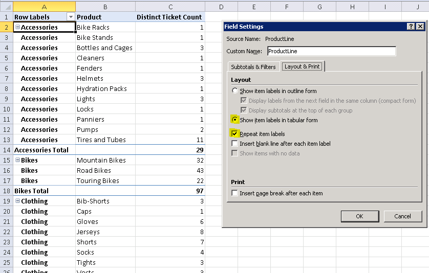
At the center of any Excel-based business intelligence solution is the PivotTable. PivotTables allow you to quickly summarize and sort information through a combination of numeric measures and row- and column-based slicers. We will assume that you have some familiarity with basic functionality of PivotTables and will focus on the features that are new or enhanced with the 2010 release of Excel. These include the ability to “Repeat Down Labels” on child members of a PivotTable, “Show Values As” a variety of calculations, filter calculated members of a cube, toggle visual totals on a PivotTable, and gain easier access to display values on rows instead of columns. See Figure 19-1.

Figure 19-1. Repeating down labels

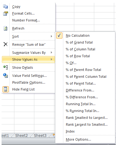
When right-clicking on a measure in a PivotTable, Excel 2010 offers one-click access to format the data via a calculation, as shown in Figure 19-2. Primarily, this is a usability improvement that makes these calculations more accessible in context. Six new calculations have also been added to create new analysis capabilities, including Percent of Parent Row Total, Percent of Parent Column Total, Percent of Parent Total from a defined parent dimension, Percent of Running Total, Rank Smallest to Largest, and Rank Largest to Smallest. We will apply these to our dataset to achieve new insights later in this chapter. Let’s try out some of the new features in our solution.

Figure 19-2. Showing no calculation in a field

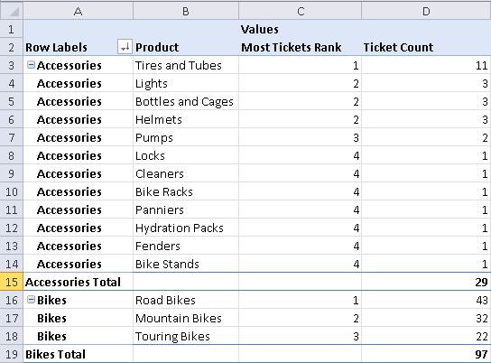
As you can see, we have applied the Rank Largest to Smallest option to column C. This ranking quickly identifies the most leveraged products in our help desk application. Figure 19-3 shows an example where we have added to the distinct count of tickets measure as Values to the pivottable and added the Product Category and Product to Rows.

Figure 19-3. Distinct count of tickets

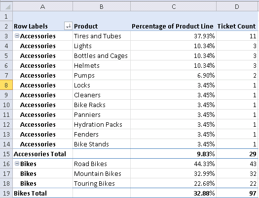
Another new transformation is the ability to show values as a percentage of the parent row. Even more then the ranking shown in the previous example, this provides new insight by showing what percentage of the total tickets for a Product Line each product received. You can imagine how this would be valuable information on its own in a pie or stacked bar chart. The process to create this is the same as the previous example except that we chose to show column C as a percentage of parent row.

Figure 19-4. Show values as a percentage

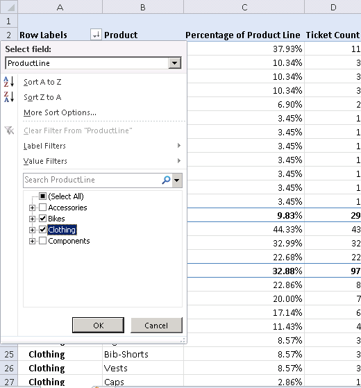
A few interesting points to share about filtering dimensions. These tips apply to dimensions that are displayed either as rows or columns. You can access the filter via the drop-down to the right of the field name, as shown in Figure 19-5. From this user interface, you can control the sort of the field in ways more sophisticated then you would think.

The More Sort Options menu item allows us to

The Label Filters provide you with the full gamut of string filtering capabilities from the basic Equals or Does Not Equal to more sophisticated Begins With, Does Not Begin With, Ends With, Does Not End With, Contains, and Does Not Contain. For the situations where your label may contain numeric information, you also have the capability to filter by Greater Than, Greater Than Or Equal To, Less Than, Less Than Or Equal To, Between, or Not Between.

Figure 19-5. Accessing PivotTable filters

When you turn to the Value Filters, the list of choices is focused just on the few numeric filters from above as we are now filtering based upon our measures. There is one great addition to the Value Filters, which is the Top X capability. This allows us to choose the top five or ten items in our pivot based on our measure.

So where might you apply this? This is great for cases such as “I want to see the five products that produce the largest number of tickets.” One might respond by saying just apply a sort and look at the top five items; why do I need a filter? The answer is that if you were to create a chart that has 50 or 100 help desk queues, your chart loses much of its impact. The unimportant data can be a distraction. This allows you as a report developer to focus the business on the items that are the most impactful data. We are a big fan of Top X, especially when used in combination with PivotCharts.

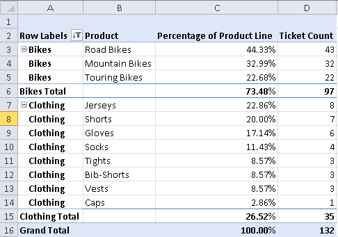
The next item is a checkbox called Include Filtered Items in Totals, but those of us who have previous experience developing multidimensional cubes will know this as visual totals. The default behavior in Excel is to provide you with visual totals. This means that when a measure is subtotaled or totaled, the filtered items are removed from the calculation. This is a great default behavior as it makes things behave the way we expect; that is, when we filter a dimension, the total reflects only the visible items. Hence the name visual totals. An example of this is shown in Figure 19-6 where we have filtered our PivotTable to show only tickets for the bikes and clothing product lines. We see that bikes have 97 tickets and clothing has 35 tickets. With the help of a calculator, we will all agree that 97+35=132. We also see that the bikes product line receives about 73 percent of the ticket volume.

Figure 19-6. Visual totals enabled for filtered product lines

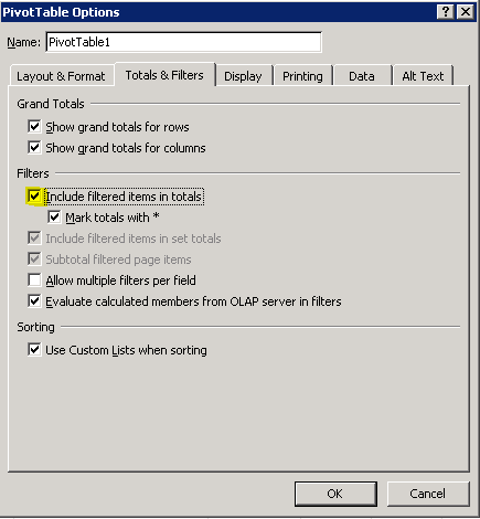
The downside of this approach is that you are missing data that can provide important context in a solution. Figure 19-7 shows us how to use the PivotTable options to disable visual totals by choosing to Include filtered items in totals.

Figure 19-7. Disabling visual totals

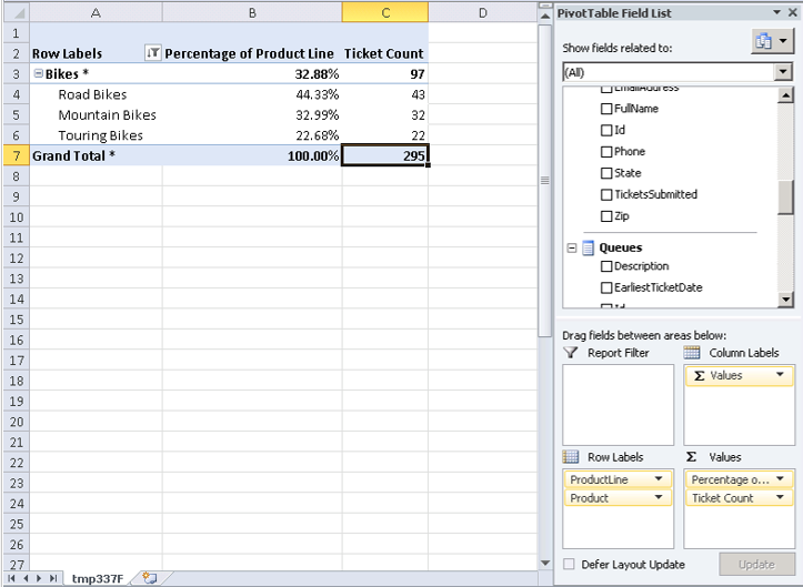
In Figure 19-8, we can see the result of disabling visual totals. The first thing to notice is that we are still filtered to display only the two product lines in which we are interested. Next, notice our measure that is showing Ticket Count as a percentage of the parent row still functions as it did before summing our visible product lines to 100%. Finally, notice that bikes ticket volume is now shown as 32.88% of the total instead of 73.48% as shown in the example with visual totals enabled. This will let us make a better informed decision by looking at our data with the relevance of the full dataset to help us. Visual totals are often useful and are a great default, but knowing how to disable them will provide an additional option when designing analytics reports.

Figure 19-8. Filtered PivotTable with visual totals disabled

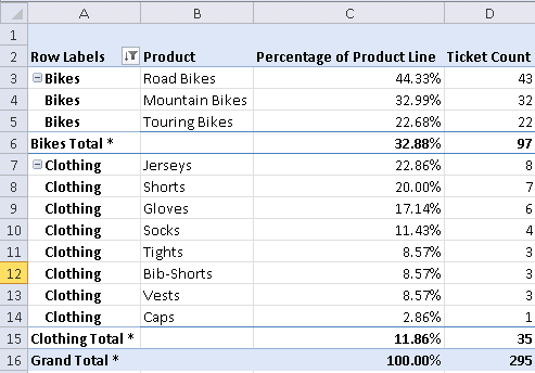
As you can see in Figure 19-9, we filtered our product line to show only bikes. The important thing to notice in this example is how smart the hierarchies are. Examining the percentages for the children of the bikes product line, we see that the percentages all add up to 100% and the ticket counts add up correctly to the total of 97 tickets that the bikes product line received. This is exactly what you would expect.

The value add with this example is that bikes formed 32.88% of the total tickets for our company, or 97/295 tickets. With visual totals enabled, we would not have had this context. You will find that developing user experiences in this toolset is not technically challenging. You do, however, need to have an idea of what capabilities the toolset provides so you can leverage it with your data.

Figure 19-9. Visual totals on filtered product like percentages

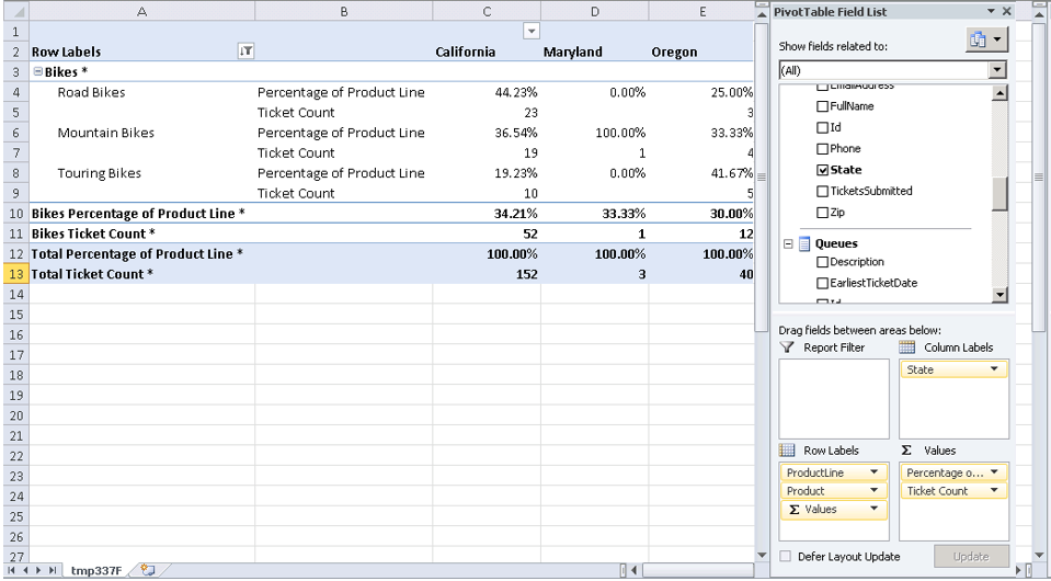
One of the more powerful capabilities of the modern Excel PivotTable is the ability to move the values (or measures) to show on rows instead of columns. Showing the values on rows is the easiest way to provide what are called OVER or BY visualizations.

In the example shown in Figure 19-10, we are showing tickets BY state. This same technique would be useful for tickets (or sales) OVER time. From a user experience perspective, our eyes find it easy to compare values that are next to each other in a row. By placing the values in the row, we are able to see a measure sliced by another measure for easy comparison.

To enable this experience, simply:

Figure 19-10. Bike sales by state

PivotTables are great! They allow us to quickly gain new insights from our data that would be unimaginably difficult if we had to do it my hand. Look at any of our previous examples to see some pretty insightful things such as ticket volume for each product by state. In a single click, we can roll that information up to a product line and gain a whole new set of information that lets us manage our business. As much as we love PivotTables and data, we all know that a picture is worth a thousand words. It takes time to understand and digest a screen full of tabular data, but a PivotChart can tell a story in just a glance.

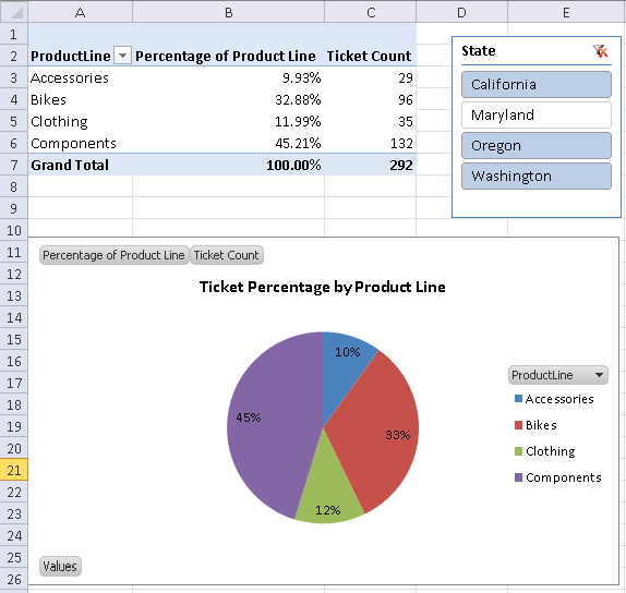
Examine the top and bottom of Figure 19-11. The pie chart on the bottom immediately communicates that components generate the majority of the support tickets, followed by bikes. Clothing and accessories seem to require very little support. While the data in the table at the top of the screen provides more detail, you may find yourself needing to pause and ask, “Sooo... what exactly am I looking at here?”

Figure 19-11. Ticket percentage by product line pie chart

Now that we agree that charts can be a useful tool to communicate information at a glance, let’s do a quick exercise to create a couple of them.

Figure 19-12. Create a PivotChart from the Ribbon.

Figure 19-13. Insert Chart Dialog.

Your chart appears below in Figure 19-14. The PivotChart is a first-class object in Excel that you can drag and drop to a new location in the workbook. You can cut and paste it to a new worksheet if needed, and you can refine the styling and layout using the controls on the Chart Design ribbon, as shown in Figure 19-14.

Figure 19-14. Chart Design Ribbon.

Take some time to explore the different chart types to find the one that best communicates your data. From a technical perspective, this couldn’t be easier.

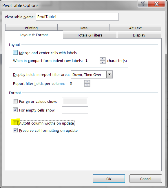
When designing a professional looking dashboard in Excel, the next tip is crucial but often overlooked. Right-click on your PivotTable and select PivotTable Options to launch the dialog shown in Figure 19-15. By default, Excel will automatically resize your column widths each time you pivot of filter the data based upon the width of the data in each column. By choosing to disable Autofit column widths on update, we can have more control over the layout of our solution and ensure it won’t change as we filter the data.

Figure 19-15. Disabling Autofit column widths on update

In this chapter, we introduced you to the basics of PivotTables and PivotCharts. Remember to disable Autofit column widths on update for improved layout control, and move values to rows for trend over time style analysis. These powerful analysis tools have made Excel the most popular application in the world for data analysis. In the next chapter, we will introduce slicers that make filtering easier and more visual.