
Particle Size Analysis
Size analysis of the various products of a concentrator is of importance in determining the quality of grinding, and in establishing the degree of liberation of the values from the gangue at various particle sizes. In the separation stage, size analysis of the products is used to determine the optimum size of the feed to the process for maximum efficiency and to determine the size range at which any losses are occurring in the plant, so that they may be reduced.
Keywords
Sieve analysis; sub-sieve techniques; data presentation; on-line analysis
4.1 Introduction
Size analysis of the various products of a concentrator is of importance in determining the quality of grinding, and in establishing the degree of liberation of the values from the gangue at various particle sizes. In the separation stage, size analysis of the products is used to determine the optimum size of the feed to the process for maximum efficiency and to determine the size range at which any losses are occurring in the plant, so that they may be reduced.
It is essential, therefore, that methods of size analysis be accurate and reliable, as important changes in plant operation may be made based on the results of these tests. Since it is often the case that only relatively small amounts of material are used in sizing tests, it is essential that the sample is representative of the bulk material and the same care should be taken over sampling for size analysis as is for assaying (Chapter 3).
4.2 Particle Size and Shape
The primary function of precision particle analysis is to obtain quantitative data about the size and size distribution of particles in the material (Bernhardt, 1994; Allen, 1997). However, exact size of an irregular particle cannot be measured. The terms “length,” “breadth,” “thickness,” or “diameter” have little meaning because so many different values of these quantities can be determined. The size of a spherical particle is uniquely defined by its diameter. For a cube, the length along one edge is characteristic, and for other regular shapes there are equally appropriate dimensions.
For irregular particles, it is desirable to quote the size of a particle in terms of a single quantity, and the expression most often used is the “equivalent diameter.” This refers to the diameter of a sphere that would behave in the same manner as the particle when submitted to some specified operation.
The assigned equivalent diameter usually depends on the method of measurement, hence the particle-sizing technique should, when possible, duplicate the type of process one wishes to control.
Several equivalent diameters are commonly encountered. For example, the Stokes’ diameter is measured by sedimentation and elutriation techniques, the projected area diameter is measured microscopically, and the sieve-aperture diameter is measured by means of sieving. The latter refers to the diameter of a sphere equal to the width of the aperture through which the particle just passes. If the particles under test are not true spheres, and they rarely are in practice, this equivalent diameter refers only to their second largest dimension.
Recorded data from any size analysis should, where possible, be accompanied by some remarks which indicate the approximate shape of the particles. Fractal analysis can be applied to particle shape. Descriptions such as “granular” or “acicular” are usually quite adequate to convey the approximate shape of the particle in question.
Some of these terms are given below:
| Acicular | Needle-shaped |
| Angular | Sharp-edged or having roughly polyhedral shape |
| Crystalline | Freely developed in a fluid medium of geometric shape |
| Dendritic | Having a branched crystalline shape |
| Fibrous | Regular or irregularly thread-like |
| Flaky | Plate-like |
| Granular | Having approximately an equidimensional irregular shape |
| Irregular | Lacking any symmetry |
| Modular | Having rounded, irregular shape |
| Spherical | Global shape |
There is a wide range of instrumental and other methods of particle size analysis available. A short list of some of the more common methods is given in Table 4.1, together with their effective size ranges (these can vary greatly depending on the technology used), whether they can be used wet or dry and whether fractionated samples are available for later analysis.
Table 4.1
Some Methods of Particle Size Analysis
| Method | Wet/Dry | Fractionated Sample? | Approx. Useful Size Range (µm)a |
| Test sieving | Both | Yes | 5–100,000 |
| Laser diffraction | Both | No | 0.1–2,500 |
| Optical microscopy | Dry | No | 0.2–50 |
| Electron microscopy | Dry | No | 0.005–100 |
| Elutriation (cyclosizer) | Wet | Yes | 5–45 |
| Sedimentation (gravity) | Wet | Yes | 1–40 |
| Sedimentation (centrifuge) | Wet | Yes | 0.05–5 |

aA micrometer (micron) (µm) is 10−6 m.
4.3 Sieve Analysis
Test sieving is the most widely used method for particle size analysis. It covers a very wide range of particle sizes, which is important in industrial applications. So common is test sieving as a method of size analysis that particles finer than about 75 µm are often referred to as being in the “sub-sieve” range, although modern sieving methods allow sizing to be carried out down to about 5 µm.
Sieve (or screen) analysis is one of the oldest methods of size analysis and is accomplished by passing a known weight of sample material through successively finer sieves and weighing the amount collected on each sieve to determine the percentage weight in each size fraction. Sieving is carried out with wet or dry materials and the sieves are usually agitated to expose all the particles to the openings. Sieving, when applied to irregularly shaped particles, is complicated by the fact that a particle with a size near that of the nominal aperture of the test sieve may pass only when presented in a favorable orientation. As there is inevitably a variation in the size of sieve apertures due to irregularity of weaving, prolonged sieving will cause the larger apertures to exert an unduly large effect on the sieve analysis. Given time, every particle small enough could find its way through a very few such holes. The procedure is also complicated in many cases by the presence of “near-size” particles which cause “blinding,” or obstruction of the sieve apertures, and reduce the effective area of the sieving medium. Blinding is most serious with test sieves of very small aperture size.
The process of sieving may be divided into two stages. The first step is the elimination of particles considerably smaller than the screen apertures, which should occur fairly rapidly. The second step is the separation of the so-called “near-size” particles, which is a gradual process rarely reaching completion. Both stages require the sieve to be manipulated in such a way that all particles have opportunities to pass through the apertures, and so that any particles that blind an aperture may be removed from it. Ideally, each particle should be presented individually to an aperture, as is permitted for the largest aperture sizes, but for most sizes this is impractical.
The effectiveness of a sieving test depends on the amount of material put on the sieve (the “charge”) and the type of movement imparted to the sieve.
A comprehensive account of sampling techniques for sieving is given in BS 1017-1 (Anon., 1989a). Basically, if the charge is too large, the bed of material will be too deep to allow each particle a chance to meet an aperture in the most favorable position for sieving in a reasonable time. The charge, therefore, is limited by a requirement for the maximum amount of material retained at the end of sieving appropriate to the aperture size. On the other hand, the sample must contain enough particles to be representative of the bulk, so a minimum size of sample is specified. In some cases, the sample will have to be subdivided into a number of charges if the requirements for preventing overloading of the sieves are to be satisfied. In some cases, air is blown through the sieves to decrease testing time and decrease the amount of blinding occurring, a technique referred to as air jet sieving.
4.3.1 Test Sieves
Test sieves are designated by the nominal aperture size, which is the nominal central separation of opposite sides of a square aperture or the nominal diameter of a round aperture. A variety of sieve aperture ranges are used, the most popular being the following: the German Standard, DIN 4188; ASTM standard, E11; the American Tyler series; the French series, AFNOR; and the British Standard, BS 1796.
Woven-wire sieves were originally designated by a mesh number, which referred to the number of wires per inch, which is the same as the number of square apertures per square inch. This has the serious disadvantage that the same mesh number on the various standard ranges corresponds to different aperture sizes depending on the thickness of wire used in the woven-wire cloth. Sieves are now designated by aperture size, which gives the user directly the information needed.
Since some workers and the older literature still refer to sieve sizes in terms of mesh number, Table 4.2 lists mesh numbers for the British Standards series against nominal aperture size. A fuller comparison of several standards is given in Napier-Munn et al. (1996).
Table 4.2
| Mesh Number | Nominal Aperture Size (µm) | Mesh Number | Nominal Aperture Size (µm) |
| 3 | 5,600 | 36 | 425 |
| 3.5 | 4,750 | 44 | 355 |
| 4 | 4,000 | 52 | 300 |
| 5 | 3,350 | 60 | 250 |
| 6 | 2,800 | 72 | 212 |
| 7 | 2,360 | 85 | 180 |
| 8 | 2,000 | 100 | 150 |
| 10 | 1,700 | 120 | 125 |
| 12 | 1,400 | 150 | 106 |
| 14 | 1,180 | 170 | 90 |
| 16 | 1,000 | 200 | 75 |
| 18 | 850 | 240 | 63 |
| 22 | 710 | 300 | 53 |
| 25 | 600 | 350 | 45 |
| 30 | 500 | 400 | 38 |

Wire-cloth screens are woven to produce nominally uniform square apertures within required tolerances (Anon., 2000a). Wire cloth in sieves with a nominal aperture of 75 µm and greater are plain woven, while those in cloths with apertures below 63 µm may be twilled (Figure 4.1).

Standard test sieves are not available with aperture sizes smaller than about 20 µm. Micromesh sieves are available in aperture sizes from 2 µm to 150 µm, and are made by electroforming nickel in square and circular mesh. Another popular type is the “micro-plate sieve,” which is fabricated by electroetching a nickel plate. The apertures are in the form of truncated cones with the small circle uppermost (Figure 4.2). This reduces blinding (a particle passing the upper opening falls away unhindered) but also reduces the percentage open area, that is, the percentage of the total area of the sieving medium occupied by the apertures.

Micro-sieves are used for wet or dry sieving where accuracy is required in particle size analysis down to the very fine size range (Finch and Leroux, 1982). The tolerances in these sieves are much better than those for woven-wire sieves, the aperture being guaranteed to within 2 µm of nominal size.
For aperture sizes above about 1 mm, perforated plate sieves are often used, with round or square holes (Figure 4.3). Square holes are arranged in line with the center points at the vertices of squares, while round holes are arranged with the centers at the apices of equilateral triangles (Anon., 2000b).

4.3.2 Choice of Sieve Sizes
In each of the standard series, the apertures of consecutive sieves bear a constant relationship to each other. It has long been realized that a useful sieve scale is one in which the ratio of the aperture widths of adjacent sieves is the square root of 2 (√2=1.414). The advantage of such a scale is that the aperture areas double at each sieve, facilitating graphical presentation of results with particle size on a log scale.
Most modern sieve series are based on a fourth root of 2 ratio (4√2=1.189) or, on the metric scale, a tenth root of 10 (10√10=1.259), which makes possible much closer sizing of particles.
For most size analyses it is usually impracticable and unnecessary to use all the sieves in a particular series. For most purposes, alternative sieves, that is, a √2 series, are quite adequate. However, over certain size ranges of particular interest, or for accurate work the ![]() series may be used. Intermediate sieves should never be chosen at random, as the data obtained will be difficult to interpret.
series may be used. Intermediate sieves should never be chosen at random, as the data obtained will be difficult to interpret.
In general, the sieve range should be chosen such that no more than about 5% of the sample is retained on the coarsest sieve, or passes the finest sieve. (The latter guideline is often difficult to meet with the finer grinds experienced today.) These limits of course may be lowered for more accurate work.
4.3.3 Testing Methods
The general procedures for test sieving are comprehensively covered in BS 1796 (Anon., 1989b). Machine sieving is almost universally used, as hand sieving is tedious, and its accuracy and precision depends to a large extent on the operator.
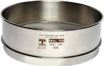
Sieves can be procured in a range of diameters, depending on the particle size and mass of material to be sieved. A common diameter for laboratory sieves is 200 mm (Figure 4.4).
The sieves chosen for the test are arranged in a stack, or nest, with the coarsest sieve on the top and the finest at the bottom. A tight-fitting pan or receiver is placed below the bottom sieve to receive the final undersize, and a lid is placed on top of the coarsest sieve to prevent escape of the sample.
The material to be tested is placed in the uppermost, coarsest sieve, and the nest is then placed in a sieve shaker, which vibrates the material in a vertical plane (Figure 4.5), and, on some models, a horizontal plane. The duration of screening can be controlled by an automatic timer. During the shaking, the undersize material falls through successive sieves until it is retained on a sieve having apertures which are slightly smaller than the diameter of the particles. In this way, the sample is separated into size fractions.

After the required time, the nest is taken apart and the amount of material retained on each sieve is weighed. Most of the near-mesh particles, which block the openings, can be removed by inverting the sieve and tapping the frame gently. Failing this, the underside of the gauze may be brushed gently with a soft brass wire or nylon brush. Blinding becomes more of a problem the finer the aperture, and brushing, even with a soft hair brush, of sieves finer than about 150 µm aperture tends to distort the individual meshes.
Wet sieving can be used on material already in the form of slurry, or it may be necessary for powders which form aggregates when dry-sieved. A full description of the techniques is given in BS 1796 (Anon., 1989b).
Water is the liquid most frequently used in wet sieving, although for materials which are water-repellent, such as coal or some sulfide ores, a wetting agent may be necessary.
The test sample may be washed down through a nest of sieves. At the completion of the test the sieves, together with the retained oversize material, are dried at a suitable low temperature and weighed.
4.3.4 Presentation of Results
There are several ways in which the results of a sieve test can be tabulated. The three most convenient methods are shown in Table 4.3 (Anon., 1989b). Table 4.3 shows for the numbered columns:
1. The sieve size ranges used in the test.
2. The weight of material in each size range. For example, 1.32 g of material passed through the 250 µm sieve, but was retained on the 180 µm sieve: the material therefore is in the size range −250 to +180 µm.
3. The weight of material in each size range expressed as a percentage of the total weight.
4. The nominal aperture sizes of the sieves used in the test.
5. The cumulative percentage of material passing through the sieves. For example, 87.5% of the material is less than 125 µm in size.
6. The cumulative percentage of material retained on the sieves.
Table 4.3
| (1) | (2) | (3) | (4) | (5) | (6) |
| Sieve Size Range (µm) | Sieve Fraction | Nominal Aperture Size (µm) | Cumulative (%) | ||
| wt (g) | wt (%) | Undersize | Oversize | ||
| +250 | 0.02 | 0.1 | 250 | 99.9 | 0.1 |
| −250 to +180 | 1.32 | 2.9 | 180 | 97.0 | 3.0 |
| −180 to +125 | 4.23 | 9.5 | 125 | 87.5 | 12.5 |
| −125 to +90 | 9.44 | 21.2 | 90 | 66.3 | 33.7 |
| −90 to +63 | 13.10 | 29.4 | 63 | 36.9 | 63.1 |
| −63 to +45 | 11.56 | 26.0 | 45 | 10.9 | 89.1 |
| −45 | 4.87 | 10.9 | |||

The results of a sieving test should always be plotted graphically to assess their full significance (Napier-Munn et al., 1996).
There are many ways of recording the results of sieve analysis, the most common being that of plotting cumulative undersize (or oversize) against particle size, that is, the screen aperture. Although arithmetic graph paper can be used, it suffers from the disadvantage that points in the region of the finer aperture sizes become congested. A semi-logarithmic plot avoids this, with a linear ordinate for percentage oversize or undersize and a logarithmic abscissa for particle size. Figure 4.6 shows graphically the results of the sieve test tabulated in Table 4.3.

It is not necessary to plot both cumulative oversize (or coarser than) and undersize (finer than) curves, as they are mirror images of each other. A valuable quantity that can be determined from such curves is the “median size” of the sample. This refers to the mid-point in the size distribution, X50, where 50% of the particles are smaller than this size and 50% are larger, also called the 50% passing size.
Size analysis is important in assessing the performance of grinding circuits. The product size is usually quoted in terms of one point on the cumulative undersize curve, this often being the 80% passing size, X80. On Figure 4.6 the X80 is about 110 µm. In a grinding circuit it is common to refer to the 80% passing size of the feed and product as F80 and P80, respectively, and to T80 as the transfer size between grinding units (e.g., SAG mill product going to a ball mill). Although the X80 does not show the overall size distribution of the material, it does facilitate routine control of the grinding circuit. For instance, if the target size is 80% −250 µm (80% finer than 250 µm), then for routine control the operator needs only screen a fraction of the mill product at one size. If it is found that, say, 70% of the sample is −250 µm, then the product is too coarse, and control steps to remedy this can be made.
Many curves of cumulative oversize or undersize against particle size are S-shaped, leading to congested plots at the extremities of the graph. More than a dozen methods of plotting in order to proportion the ordinate are known. The two most common methods, which are often applied to comminution studies where non-uniform size distributions are obtained, are the Gates-Gaudin-Schuhmann (Schuhmann, 1940) and the Rosin–Rammler (Rosin and Rammler, 1933) methods. Both methods are derived from attempts to represent particle size distribution curves by means of equations. This results in scales which, relative to a linear scale, are expanded in some regions and contracted in others.
In the Gates-Gaudin-Schuhmann (G-G-S) method, cumulative undersize data are plotted against sieve aperture on log–log axes. This frequently leads to a linear trend from which data can be interpolated easily. The linear trend is fitted to the following:
(4.1)
which can be written as:
(4.2)
where P is the cumulative undersize (or passing) in percent, X the particle size, K the apparent (theoretical) top size (i.e., when P=100%) obtained by extrapolation, and α a constant sometimes referred to as the distribution coefficient (Austin et al., 1984). This method of plotting is routinely used in grinding studies (laboratory and plant). An example G-G-S plot is shown in Figure 4.7 for increased grinding time in a laboratory ball mill (data given in Appendix IV). The figure shows a series of roughly parallel (or self-similar) linear sections of the size distributions. This result, showing a consistent behavior, is quite common in grinding (and other) studies (but see Chapter 5 for exceptions) and supports the use of a single metric to describe the distribution, for example, the 80% passing size, X80 (Austin et al., 1984).

Self-similar distributions such as in Figure 4.7 become a unique distribution by plotting against a reduced particle size, typically X/X50 where X50 is the 50% passing size or median size. If it is known that data obtained from the material usually yield a linear plot on log–log axes, then the burden of routine analysis can be greatly relieved, as relatively few sieves will be needed to check essential features of the size distribution. Self-similarity can be quickly identified, as a plot of, say, %−75 µm versus % +150 µm will yield a single curve if this property holds.
Plotting on a log–log scale considerably expands the region below 50% in the cumulative undersize curve, especially that below 25%. It does, however, severely contract the region above 50%, and especially above 75%, which is a disadvantage of the method (Figure 4.8).

The Rosin–Rammler method is often used for representing the results of sieve analyses performed on material which has been ground in ball mills. Such products have been found to obey the following relationship (Austin et al., 1984):
(4.3)
where b and n are constants.
This can be rewritten as:
(4.4)
Thus, a plot of ln [100/(100–P)] versus X on log–log axes gives a line of slope n.
In comparison with the log–log method, the Rosin–Rammler plot expands the cumulative undersize regions below 25% and above 75% (Figure 4.8) and it contracts the 30–60% region. It has been shown, however, that this contraction is insufficient to cause adverse effects (Harris, 1971). The method is tedious to plot manually unless charts having the axes divided proportionally to log [ln (100/(100–P))] and log X are used. The data can, however, be easily plotted in a spreadsheet.
The Gates-Gaudin-Schuhmann plot is often preferred to the Rosin–Rammler method in mineral processing applications, the latter being more often used in coal-preparation studies, for which it was originally developed. The two methods have been assessed by Harris (1971), who suggests that the Rosin–Rammler is the better method for mineral processing applications. The Rosin–Rammler is useful for monitoring grinding operations for highly skewed distributions, but, as noted by Allen (1997), it should be used with caution, since taking logs always apparently reduces scatter, and thus taking logs twice is not to be recommended.
Although cumulative size curves are used almost exclusively, the particle size distribution curve itself is sometimes more informative. Ideally, this is derived by differentiating the cumulative undersize curve and plotting the gradient of the curve obtained against particle size. In practice, the size distribution curve is obtained by plotting the retained fraction of the sieves against size. This can be as a histogram or as a frequency (fractional) curve plotted at the “average” size in between two sieve sizes. For example, material which passes a 250 µm sieve but is retained on a 180 µm sieve, may be regarded as having an arithmetic mean particle size of 215 µm or, more appropriately since the sieves are in a geometric sequence, a geometric mean (√(250×180)) of 212 µm for the purpose of plotting. If the distribution is represented on a histogram, then the horizontals on the columns of the histogram join the various adjacent sieves used in the test. Unless each size increment is of equal width, however, the histogram has little value. Figure 4.9 shows the size distribution of the material in Table 4.3 represented on a frequency curve and a histogram.

Fractional curves and histograms are useful and rapid ways of visualizing the relative frequency of occurrence of the various sizes present in the material. The only numerical parameter that can be obtained from these methods is the “mode” of the distribution, that is, the most commonly occurring size.
For assessment of the metal losses in the tailings of a plant, or for preliminary evaluation of ores, assaying must be carried out on the various screen fractions. It is important, therefore, that the bulk sample satisfies the minimum sample weight requirement given by Gy’s equation for the fundamental error (Chapter 3).
Table 4.4 shows the results of a screen analysis performed on an alluvial tin deposit for preliminary evaluation of its suitability for treatment by gravity concentration. Columns 1, 2, and 3 show the results of the sieve test and assays, which are evaluated in the other columns. It can be seen that the calculated overall assay for the material is 0.21% Sn, but that the bulk of the tin is present within the finer fractions. The results show that, for instance, if the material was initially screened at 210 µm and the coarse fraction discarded, then the bulk required for further processing would be reduced by 24.9%, with a loss of only 4.6% of the Sn. This may be acceptable if mineralogical analysis shows that the tin is finely disseminated in this coarse fraction, which would necessitate extensive grinding to give reasonable liberation. Heavy liquid analysis (Chapter 11) on the −210 µm fraction would determine the theoretical (i.e., liberation-limited, Chapter 1) grades and recoveries possible, but the screen analysis results also show that much of the tin (22.7%) is present in the −75 µm fraction, which constitutes only 1.9% of the total bulk of the material. This indicates that there may be difficulty in processing this material, as gravity separation techniques are not very efficient at such fine sizes (Chapters 1 and 10).
Table 4.4
Results of Screen Analysis to Evaluate the Suitability for Treatment by Gravity Concentration
| (1) Size Range (µm) | (2) Weight (%) | (3) Assay (% Sn) | Distribution (% Sn) | Size (µm) | Cumulative oversize (Wt %) | Cumulative distribution (% Sn) |
| +422 | 9.7 | 0.02 | 0.9 | 422 | 9.7 | 0.9 |
| −422 + 300 | 4.9 | 0.05 | 1.2 | 300 | 14.6 | 2.1 |
| −300 + 210 | 10.3 | 0.05 | 2.5 | 210 | 24.9 | 4.6 |
| −210 + 150 | 23.2 | 0.06 | 6.7 | 150 | 48.1 | 11.3 |
| −150 + 124 | 16.4 | 0.12 | 9.5 | 124 | 64.5 | 20.8 |
| −124 + 75 | 33.6 | 0.35 | 56.5 | 75 | 98.1 | 77.3 |
| −75 | 1.9 | 2.50 | 22.7 | |||
| 100.0 | 0.21 | 100.0 |

4.4 Sub-sieve Techniques
Sieving is rarely carried out on a routine basis below 38 µm; below this size the operation is referred to as sub-sieving. The most widely used methods are sedimentation, elutriation, microscopy, and laser diffraction, although other techniques are available.
There are many concepts in use for designating particle size within the sub-sieve range, and it is important to be aware of them, particularly when combining size distributions determined by different methods. It is preferable to cover the range of a single distribution with a single method, but this is not always possible.
Conversion factors between methods will vary with sample characteristics and conditions, and with size where the distributions are not self-similar. For spheres, many methods will give essentially the same result (Napier-Munn, 1985), but for irregular particles this is not so. Some approximate factors for a given characteristic size (e.g., X80) are given below (Austin and Shah, 1983; Napier-Munn, 1985; Anon., 1989b)—these should be used with caution:
| Conversion | Multiplying Factor |
| Sieve size to Stokes’ diameter (sedimentation, elutriation) | 0.94 |
| Sieve size to projected area diameter (microscopy) | 1.4 |
| Sieve size to laser diffraction | 1.5 |
| Square mesh sieves to round hole sieves | 1.2 |
4.4.1 Stokes’ Equivalent Diameter
In sedimentation techniques, the material to be sized is dispersed in a fluid and allowed to settle under carefully controlled conditions; in elutriation techniques, samples are sized by allowing the dispersed material to settle against a rising fluid velocity. Both techniques separate the particles on the basis of resistance to motion in a fluid. This resistance to motion determines the terminal velocity which the particle attains as it is allowed to fall in a fluid under the influence of gravity.
For particles within the sub-sieve range, the terminal velocity is given by the equation derived by Stokes (1891):
(4.5)
where v is the terminal velocity of the particle (m s−1), d the particle diameter (m), g the acceleration due to gravity (m s−2), ρs the particle density (kg m−3), ρf the fluid density (kg m−3), and η the fluid viscosity (N s m−2); (η=0.001 N s m−2 for water at 20°C).
Stokes’ law is derived for spherical particles; non-spherical particles will also attain a terminal velocity, but this velocity will be influenced by the shape of the particles. Nevertheless, this velocity can be substituted in the Stokes’ equation to give a value of d, which can be used to characterize the particle. This value of d is referred to as the “Stokes’ equivalent spherical diameter” (or simply “Stokes’ diameter” or “sedimentation diameter”).
Stokes’ law is only valid in the region of laminar flow (Chapter 9), which sets an upper size limit to the particles that can be tested by sedimentation and elutriation methods in a given liquid. The limit is determined by the particle Reynolds number, a dimensionless quantity defined by:
(4.6)
The Reynolds number should not exceed 0.2 if the error in using Stokes’ law is not to exceed 5% (Anon., 2001a). In general, Stokes’ law will hold for all particles below 40 µm dispersed in water; particles above this size should be removed by sieving beforehand. The lower limit may be taken as 1 µm, below which the settling times are too long, and also the effects of Brownian motion and unintentional disturbances, such as those caused by convection currents, are far more likely to produce serious errors.
4.4.2 Sedimentation Methods
Sedimentation methods are based on the measurement of the rate of settling of the powder particles uniformly dispersed in a fluid and the principle is well illustrated by the common laboratory method of “beaker decantation.”
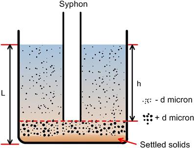
The material under test is uniformly dispersed in low concentration in water contained in a beaker or similar parallel-sided vessel. A wetting agent may need to be added to ensure complete dispersion of the particles. A syphon tube is immersed into the water to a depth of h below the water level, corresponding to about 90% of the liquid depth L.
The terminal velocity v is calculated from Stokes’ law for the various sizes of particle in the material, say 35, 25, 15, and 10 µm. For a distribution, it is usual to fix ds for the particles that are most abundant in the sample.
The time required for a 10 µm particle to settle from the water level to the bottom of the syphon tube, distance h, is calculated (t=h/v). The pulp is gently stirred to disperse the particles through the whole volume of water and then it is allowed to stand for the calculated time. The water above the end of the tube is syphoned off and all particles in this water are assumed to be smaller than 10 µm diameter (Figure 4.10). However, a fraction of the −10 µm material, which commenced settling from various levels below the water level, will also be present in the material below the syphon level. In order to recover these particles, the pulp remaining must be diluted with water to the original level, and the procedure repeated until the decant liquor is essentially clear. In theory, this requires an infinite number of decantations, but in practice at least five treatments are usually sufficient, depending on the accuracy required. The settled material can be treated in a similar manner at larger separating sizes, that is, at shorter decanting times, until a target number of size fractions is obtained.
The method is simple and cheap, and has an advantage over many other sub-sieve techniques in that it produces a true fractional size analysis, that is, reasonable quantities of material in specific size ranges are collected, which can be analyzed chemically and mineralogically.
This method is, however, extremely tedious, as long settling times are required for very fine particles, and separate tests must be performed for each particle size. For instance, a 25 µm particle of quartz has a settling velocity of 0.056 cm s−1, and therefore takes about 3½ min to settle 12 cm, a typical immersion depth for the syphon tube. Five separate tests to ensure a reasonably clear decant therefore require a total settling time of about 18 min. A 5 µm particle, however, has a settling velocity of 0.0022 cm s−1, and therefore takes about 1½ h to settle 12 cm. The total time for evaluation of such material is thus about 8 h. A complete analysis may therefore take an operator several days.
Another problem is the large quantity of water, which dilutes the undersize material, due to repeated decantation.
In the system shown in Figure 4.10, after time t, all particles larger than size d have fallen to a depth below the level h. All particles of a size d1, where d1 < d, will have fallen below a level h1 below the water level, where h1 < h. The efficiency of removal of particles of size d1 into the decant is thus:
since at time t=0 the particles were uniformly distributed over the whole volume of liquid, corresponding to depth L, and the fraction removed into the decant is the volume above the syphon level, h – h1.
Now, since t=h/v, and v ∝ d2,
Therefore, the efficiency of removal of particles of size d1
where a=h/L.
If a second decantation step is performed, the amount of minus d1 material in the dispersed suspension is 1 – E, and the efficiency of removal of minus d1 particles after two decantations is thus:
In general, for n decantation steps the efficiency of removal of particles of size d1, at a separation size of d, is:
(4.7)
Table 4.5 shows the number of decantation steps required for different efficiencies of removal of various sizes of particle expressed relative to d, the separating size, where the value of a=0.9. It can be shown (Heywood, 1953) that the value of a has relatively little effect; therefore there is nothing to be gained by attempting to remove the suspension adjacent to the settled particles, thus risking disturbance and re-entrainment.
Table 4.5
Number of Decantations Required for Required Efficiency of Removal of fine Particles
| Relative Particle Size (d1/d) | 0.95 | 0.9 | 0.8 | 0.5 | 1 | |
| Number of decantations | 90% Efficiency | 25 | 12 | 6 | 2 | 1 |
| 95% Efficiency | 33 | 16 | 8 | 3 | 1 | |
| 99% Efficiency | 50 | 25 | 12 | 4 | 2 | |
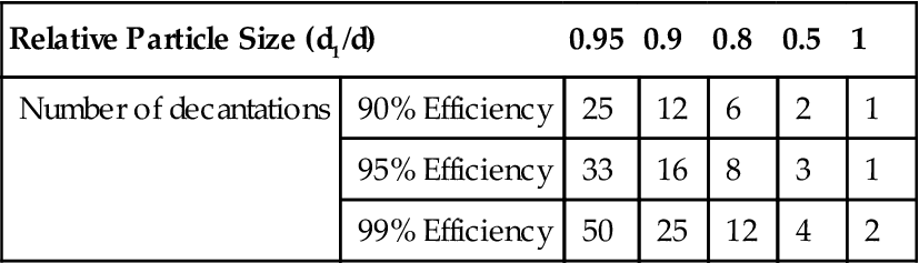
Table 4.5 shows that a large number of decantations are necessary for effective removal of particles close to the separation size, but that relatively small particles are quickly eliminated. For most purposes, unless very narrow size ranges are required, no more than about twelve decantations are necessary for the test.
A much quicker and less-tedious method of sedimentation analysis is the Andreasen pipette technique (Anon., 2001b).
The apparatus (Figure 4.11) consists of a half-liter graduated cylindrical flask and a pipette connected to a 10 mL reservoir by means of a two-way stop-cock. The tip of the pipette is in the plane of the zero mark when the ground glass stopper is properly seated.

A 3 to 5% suspension of the sample, dispersed in the sedimentation fluid, usually water, is added to the flask. The pipette is introduced and the suspension agitated by inversion. The suspension is then allowed to settle, and at given intervals of time, samples are withdrawn by applying suction to the top of the reservoir, manipulating the two-way cock so that the sample is drawn up as far as the calibration mark on the tube above the 10 mL reservoir. The cock is then reversed, allowing the sample to drain into the collecting dish. After each sample is taken, the new liquid level is noted.
The samples are then dried and weighed, and the weights compared with the weight of material in the same volume of the original suspension.
There is a definite particle size, d, corresponding to each settling distance h and time t, and this represents the size of the largest particle that can still be present in the sample. These particle sizes are calculated from Stokes’ law for the various sampling times. The weight of solids collected, w, compared with the corresponding original weight, wo (i.e., w/wo) then represents the fraction of the original material having a particle size smaller than d, which can be plotted on the size-analysis graph.
The Andreasen pipette method is quicker than beaker decantation, as samples are taken off successively throughout the test for increasingly finer particle sizes. For example, although 5 µm particles of quartz will take about 2½ h to settle 20 cm, once this sample is collected, all the coarser particle-size samples will have been taken, and so the complete analysis, in terms of settling times, is only as long as the settling time for the finest particles.
The disadvantage of the method is that the samples taken are each representative of the particles smaller than a particular size, which is not as valuable, for mineralogical and chemical analysis, as samples of various size ranges, as are produced by beaker decantation.
Sedimentation techniques tend to be tedious, due to the long settling times required for fine particles and the time required to dry and weigh the samples. The main difficulty, however, lies in completely dispersing the material within the suspending liquid, such that no agglomeration of particles occurs. Combinations of suitable suspending liquids and dispersing agents for various materials are given in BS ISO 13317–1 (Anon., 2001a).
Various other techniques have been developed that attempt to speed up testing. Examples of these methods, which are comprehensively reviewed by Allen (1997), include: the photo-sedimentometer, which combines gravitational settling with photo-electric measurement; and the sedimentation balance, in which the weight of material settling out onto a balance pan is recorded against time to produce a cumulative sedimentation size analysis.
4.4.3 Elutriation Techniques
Elutriation is a process of sizing particles by means of an upward current of fluid, usually water or air. The process is the reverse of gravity sedimentation, and Stokes’ law applies.
All elutriators consist of one or more “sorting columns” (Figure 4.12) in which the fluid is rising at a constant velocity. Feed particles introduced into the sorting column will be separated into two fractions, according to their terminal velocities, calculated from Stokes’ law.
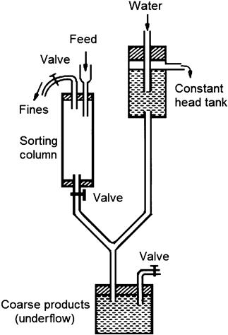
Those particles having a terminal velocity less than that of the velocity of the fluid will report to the overflow, while those particles having a greater terminal velocity than the fluid velocity will sink to the underflow. Elutriation is carried out until there are no visible signs of further classification taking place or the rate of change in weights of the products is negligible.
An elutriator based on air is the Haultain infrasizer, which comprises six sorting columns (”cones”) plus a dust collector (Price, 1962). More commonly, water is the fluid. This involves the use of much water and dilution of the undersize fraction, but it can be shown that this is not as serious as in beaker decantation. Consider a sorting column of depth h, sorting material at a separating size of d. If the upward velocity of water flow is v, then (as noted above) by Stokes’ law, v ∝ d2.
Particles smaller than the separating size d will move upwards in the water flow at a velocity dependent on their size. Thus, particles of size d1, where d1 < d, will move upwards in the sorting column at a velocity v1, where ![]() .
.
The time required for a complete volume change in the sorting column is h/v, and the time required for particles of size d1 to move from the bottom to the top of the sorting column is h/v1. Therefore, the number of volume changes required to remove all particles of size d1 from the sorting column is:
and the number of volume changes required for various values of d1/d are:
| d1/d | 0.95 | 0.9 | 0.8 | 0.5 | 0.1 |
| Number of volume changes required | 10.3 | 5.3 | 2.8 | 1.3 | 1.0 |

Comparing these figures with those in Table 4.5, it can be seen that the number of volume changes required is far less with elutriation than it is with decantation. It is also possible to achieve complete separation by elutriation, whereas this can only be achieved in beaker decantation by an infinite number of volume changes.
Elutriation thus appears more attractive than decantation, and has certain practical advantages in that the volume changes need no operator attention. It suffers from the disadvantage, however, that the fluid velocity is not constant across the sorting column, being a minimum at the walls of the column, and a maximum at the center. The separation size is calculated from the mean volume flow, so that some coarse particles are misplaced in the overflow, and some fines are misplaced into the underflow. The fractions thus have a considerable overlap in particle size and are not sharply separated. Although the decantation method never attains 100% efficiency of separation, the lack of sharpness of the division into fractions is much less than that due to velocity variation in elutriation (Heywood, 1953).
Elutriation is limited at the coarsest end by the validity of Stokes’ law, but most materials in the sub-sieve range exhibit laminar flow. At the fine end of the scale, separations become impracticable below about 10 µm, as the material tends to agglomerate, or extremely long separating times are required. Separating times can be considerably decreased by utilizing centrifugal forces. One of the most widely used methods of sub-sieve sizing in mineral processing laboratories is the Warman cyclosizer (Finch and Leroux, 1982), which is extensively used for routine testing and plant control in the size range 8–50 µm for materials of specific gravity similar to quartz (s. g. 2.7), and down to 4 µm for particles of high specific gravity, such as galena (s. g. 7.5).
The cyclosizer unit consists of five cyclones (see Chapter 9 for a full description of the principle of the hydrocyclone), arranged in series such that the overflow of one unit is the feed to the next unit (Figure 4.13).

The individual units are inverted in relation to conventional cyclone arrangements, and at the apex of each, a chamber is situated so that the discharge is effectively closed (Figure 4.14).

Water is pumped through the units at a controlled rate, and a weighed sample of solids is introduced ahead of the cyclones.
The tangential entry into the cyclones induces the liquid to spin, resulting in a portion of the liquid, together with the faster-settling particles, reporting to the apex opening, while the remainder of the liquid, together with the slower settling particles, is discharged through the vortex outlet and into the next cyclone in the series. There is a successive decrease in the inlet area and vortex outlet diameter of each cyclone in the direction of the flow, resulting in a corresponding increase in inlet velocity and an increase in the centrifugal forces within the cyclone. This results in a successive decrease in the limiting particle-separation size of the cyclones.
The cyclosizer is manufactured to have definite limiting separation sizes at standard values of the operating variables, viz. water flow rate, water temperature, particle density, and elutriation time. To correct for practical operation at other levels of these variables, a set of correction graphs is provided.
Complete elutriation normally takes place after about 20 min, at which time the sized fractions are collected by discharging the contents of each apex chamber into separate beakers. The samples are dried, and weighed to determine the mass fractions of each particle size.
4.4.4 Microscopic Sizing and Image Analysis
Microscopy can be used as an absolute method of particle size analysis, since it is the only method in which individual mineral particles are observed and measured (Anon., 1993; Allen, 1997). The image of a particle seen in a microscope is two-dimensional and from this image an estimate of particle size must be made. Microscopic sizing involves comparing the projected area of a particle with the areas of reference circles, or graticules, of known sizes, and it is essential for meaningful results that the mean projected areas of the particles are representative of the particle size. This requires a random orientation in three dimensions of the particle on the microscope slide, which is unlikely in most cases.
The optical microscope method is applicable to particles in the size range 0.8–150 µm, and down to 0.001 µm using electron microscopy.
Basically, all microscopy methods are carried out on extremely small laboratory samples, which must be collected with great care in order to be representative of the process stream under study.
In manual optical microscopy, the dispersed particles are viewed by transmission, and the areas of the magnified images are compared with the areas of circles of known sizes inscribed on a graticule.
The relative numbers of particles are determined in each of a series of size classes. These represent the size distribution by number from which it is possible to calculate the distribution by volume and, if all the particles have the same density, the distribution by weight.
Manual analysis of microscope slides is tedious and error prone; semi-automatic and automatic systems have been developed which speed up analyses and reduce the tedium of manual methods (Allen, 1997).
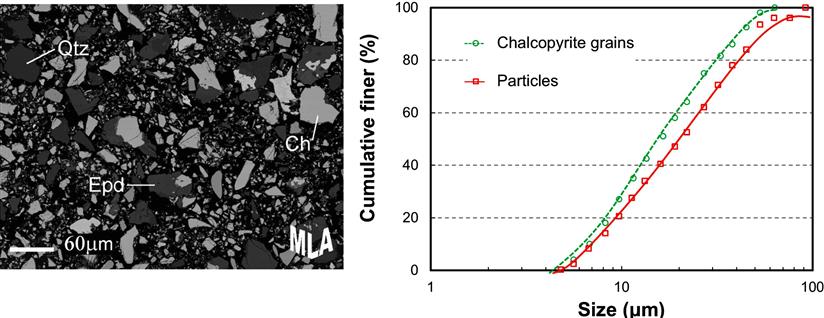
The development of quantitative image analysis has made possible the rapid sizing of fine particles. Image analyzers accept samples in a variety of forms—photographs, electron micrographs, and direct viewing—and are often integrated in system software. Figure 4.15 shows the grayscale electron backscatter image of a group of mineral particles obtained with a scanning electron microscope; grains of chalcopyrite (Ch), quartz (Qtz), and epidote (Epd) are identified in the image. On the right are plotted the size distributions of the “grains” of the mineral chalcopyrite (i.e., the pieces of chalcopyrite identified by the instrument, whether liberated or not) and the “particles” in which the chalcopyrite is present. The plots are based on the analysis of several hundred thousand particles in the original sample, and are delivered automatically by the system software. Image analysis of this kind is available in many forms for the calculation of many quantities (such as size, surface area, boundary lengths) for most imaging methods, for example, optical, electron. (See also Chapter 17.)
4.4.5 Electrical Impedance Method
The Beckman Coulter Counter makes use of current changes in an electrical circuit produced by the presence of a particle. The measuring system of a Coulter Counter is shown in Figure 4.16.

The particles, suspended in a known volume of electrically conductive liquid, flow through a small aperture having an immersed electrode on either side; the particle concentration is such that the particles traverse the aperture substantially one at a time.
Each particle passage displaces electrolyte within the aperture, momentarily changing the resistance between the electrodes and producing a voltage pulse of magnitude proportional to particle volume. The resultant series of pulses is electronically amplified, scaled, and counted.
The amplified pulses are fed to a threshold circuit having an adjustable screen-out voltage level, and those pulses which reach or exceed this level are counted, this count representing the number of particles larger than some determinable volume proportional to the appropriate threshold setting. By taking a series of counts at various amplification and threshold settings, data are directly obtained for determining number frequency against volume, which can be used to determine the size distribution.
As the instrument measures particle volume, the equivalent diameter is calculated from that of a sphere of the same volume, which can be a more relevant size measure than some alternatives. The instrument is applicable in the range 0.4–1,200 µm.
4.4.6 Laser Diffraction Instruments
In recent years, several instruments based on the diffraction of laser light by fine particles have become available, including the Malvern Master-Sizer and the Microtrac. The principle is illustrated in Figure 4.17. Laser light is passed through a dilute suspension of the particles which circulate through an optical cell. The light is scattered by the particles, which is detected by a solid state detector which measures light intensity over a range of angles. A theory of light scattering is used to calculate the particle size distribution from the light distribution pattern, finer particles inducing more scatter than coarser particles. The early instruments used Fraunhofer theory, which is suitable for coarse particles in the approximate range 1–2,000 µm (the upper limit being imposed mainly by mechanical constraints). More recently Mie theory has been used to extend the capability down to 0.1 µm and below. Some modern instruments offer both options to cover a wide size range.

Laser diffraction instruments are fast, easy to use, and give reproducible results. However, light scattering theory does not give a definition of size that is compatible with other methods, such as sieving. In most mineral processing applications, for example, laser diffraction size distributions tend to appear coarser than those of other methods. Austin and Shah (1983) have suggested a procedure for inter-conversion of laser diffraction and sieve-size distributions, and a simple conversion can be developed by regression for materials of consistent characteristics. In addition, the results can depend on the relative refractive indices of the solid particles and liquid medium (usually, though not necessarily, water), and even particle shape. Most instruments claim to compensate for these effects, or offer calibration inputs to the user.
For these reasons, laser diffraction size analyzers should be used with caution. For routine high volume analyses in a fixed environment in which only changes in size distribution need to be detected, they probably have no peer. For comparison across several environments or materials, or with data obtained by other methods, care is needed in interpreting the data. These instruments do not, of course, provide fractionated samples for subsequent analysis.
4.5 On-line Particle Size Analysis
The major advantage of on-line analysis systems is that by definition they do not require sampling by operations personnel, eliminating one source of error. They also provide much quicker results, in the case of some systems continuous measurement, which in turn decreases production delays and improves efficiency. For process control on-line measurement is essential.
4.5.1 Slurry Systems
While used sometimes on final concentrates, such as Fe concentrates, to determine the Blaine number (average particle size deduced from surface area), and on tailings for control of paste thickeners, for example, the prime application is on cyclone overflow for grinding circuit control (Kongas and Saloheimo, 2009). Control of the grinding circuit to produce the target particle size distribution for flotation (or other mineral separation process) at target throughput maximizes efficient use of the installed power.
Continuous measurement of particle size in slurries has been available since 1971, the PSM (particle size monitor) system produced then by Armco Autometrics (subsequently by Svedala and now by Thermo Gamma-Metrics) having been installed in a number of mineral processing plants (Hathaway and Guthnals, 1976).
The PSM system uses ultrasound to determine particle size. This system consists of three sections: the air eliminator, the sensor section, and the electronics section. The air eliminator draws a sample from the process stream and removes entrained air bubbles (which otherwise act as particles in the measurement). The de-aerated pulp then passes between the sensors. Measurement depends on the varying absorption of ultrasonic waves in suspensions of different particle sizes. Since solids concentration also affects the absorption, two pairs of transmitters and receivers, operating at different frequencies, are employed to measure particle size and solids concentration of the pulp, the processing of this information being performed by the electronics. The Thermo GammaMetrics PSM-400MPX (Figure 4.18) handles slurries up to 60% w/w solids and outputs five size fractions simultaneously.

Other measurement principles are now in commercial form for slurries. Direct mechanical measurement of particle size between a moving and fixed ceramic tip, and laser diffraction systems are described by Kongas and Saloheimo (2009). Two recent additions are the CYCLONEtrac systems from CiDRA Minerals Processing (Maron et al., 2014), and the OPUS ultrasonic extinction system from Sympatec (Smith et al., 2010).
CiDRA’s CYCLONEtrac PST (particle size tracking) system comprises a hardened probe that penetrates into the cyclone overflow pipe to contact the stream and effectively “listens” to the impacts of individual particles. The output is % above (or below) a given size and has been shown to compare well with sieve sizing (Maron et al., 2014). The OPUS ultrasonic extinction system (USE) transmits ultrasonic waves through a slurry that interact with the suspended particles. The detected signal is converted into a particle size distribution, the number of frequencies used giving the number of size classes measured. Applications on ores can cover a size range from 1 to 1,000 μm (Smith et al., 2010).
In addition to particles size, recent developments have included sensors to detect malfunctioning cyclones. Westendorf et al. (2015) describe the use of sensors (from Portage Technologies) on cyclone overflow and underflow piping. CiDRA’s CYCLONEtrac OSM (oversize monitor) is attached to the outside of the cyclone overflow pipe and detects the acoustic signal as oversize particles (“rocks”) hit the pipe (Cirulis and Russell, 2011). The systems are readily installed on individual cyclones thus permitting poorly operating units to be identified and changed while allowing the cyclone battery to remain in operation. Figure 4.19 shows an installation of both CiDRA systems (PST, OSM) on the overflow pipe from a cyclone.

4.5.2 On-belt Systems
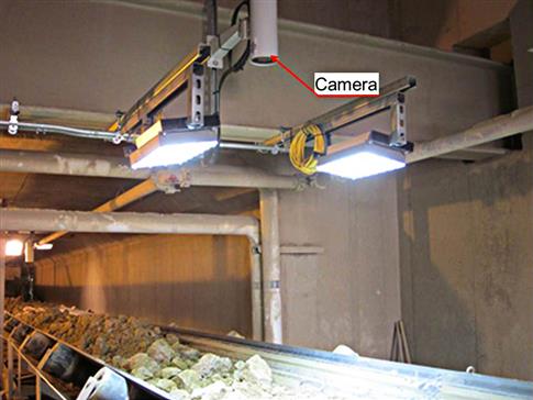
Image analysis is used in sizing rocks on conveyor belts. Systems available include those supplied by Split Engineering, WipFrag, Metso, and Portage Technologies (see also Chapter 6). A fixed camera with appropriate lighting captures images of the particles on the belt. Then, software segments the images, carries out appropriate corrections, and calculates the particle size distribution. A system installed on a conveyor is shown in Figure 4.20. Figure 4.21 shows the original camera views and the segmented images for a crusher feed and product, together with the calculated size distributions. (Another example is given in Chapter 6.) Common problems with imaging systems are the inability to “see” particles under the top layer, and the difficulty of detecting fines, for which correction algorithms can be used. The advantage of imaging systems is that they are low impact, as it possible to acquire size information without sampling or interacting with the particles being measured. These systems are useful in detecting size changes in crusher circuits, and are increasingly used in measuring the feed to SAG mills for use in mill control (Chapter 6), and in mining applications to assess blast fragmentation.

There are other on-line systems available or under test. For example, CSIRO has developed a version of the ultrasonic attenuation principle, in which velocity spectrometry and gamma-ray transmission are incorporated to produce a more robust measurement in the range 0.1–1,000 µm (Coghill et al., 2002). Most new developments in on-line analysis are modifications and improvements of previous systems, or adaptations of off-line systems for on-line usage.