
A tracer test is most readily performed on the liquid; for example, adding a salt (usually NaCl) and monitoring the conductivity on the discharge, or introducing a colored dye and monitoring the discharge using spectroscopy. Guidelines are given by Nesset (1988). Particle mixing can be determined by introducing a different type of particle to those in the flotation feed but of similar size and density; or, better, by radioactive tagging an element in the feed particles (Yianatos, 2007).
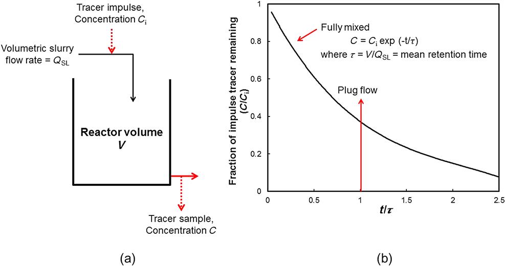
Transport exhibits two extremes: plug flow, and fully (or perfectly) mixed flow (Figure 12.32b). In plug flow all the particles enter and leave the cell at the same time, the time corresponding to the mean residence (retention) time. The mean residence time τ is given by the cell volume (m3) (with allowance for volume occupied by gas) divided by the volumetric flowrate through the cell (m3 min−1); the time scale can then be given as t/τ (a reduced or normalized time), as in Figure 12.32. Plug flow, therefore, is indicated by a (theoretical) line at t/τ=1. Fully mixed transport, on the other hand, means the tracer is immediately evenly distributed throughout the cell and thus the zero-time sample is the cell average concentration. With time the concentration decays exponentially, giving a distribution of residence times or residence time distribution (RTD).
The two extreme cases offer mathematical simplicity, which is why they are the usual starting point. The two solutions are:
The plug flow solution is the same as for the batch case, as all particles have the same residence time (at least those in the tailings stream from the cell). Equation (12.28) is derived in Appendix V.
Mechanical cells and flotation columns show an RTD close to fully mixed (Yianatos, 2007; Govender et al., 2014). While mean particle residence time depends on particle mass (size and density), it is generally close enough to the liquid mean residence time (within 90%) for most practical purposes and the simpler determination of liquid residence time suffices.
RTD studies have diagnostic value. If, for example, there is significant short circuiting, the RTD will exhibit unusual shapes; for example, more than one maxima and/or a tail extending to long times (>2.5 t/τ). RTD studies on flotation columns baffled into vertical sections revealed pulp flowing between the sections created by uneven distribution of feed and air.
12.9.3 Components of the Rate Constant
The rate constant is a function of contributions by the machine, the particles, and the froth.
Machine
The machine is responsible for production of bubble swarms and effecting bubble–particle collision. Recent work has related the machine “factor” to the BSAF. BSAF (Sb) is the rate at which bubble surface area moves through the cell per unit of cell cross-sectional area with units m2 m−2 s−1 or simply s−1. Introduced in Section 12.5, to remind, it is estimated from the measurements of superficial gas velocity (the volumetric gas flowrate per unit area of cell, Jg), and the bubble size, usually taken as the Sauter mean diameter (D32):
(12.7)
Since Jg is typically quoted in cm s−1 D32 must be in cm. To give a sense of magnitude, at a typical value of Jg=1 cm s−1 and D32=1 mm (0.1 cm) then Sb=60 s−1.
Both Jg and D32 are measurable using suitable probes (see Section 12.14.2). The Sb can also be predicted using a correlation developed by Gorain et al. (1999).
Gorain et al. (1997) and Alexander et al. (2000) showed for shallow froth depths that the first order rate constant was linearly related to the BSAF. In addition, this relationship was shown to be independent of cell size and operating parameters. This independence is illustrated in Figure 12.33, which shows that the relationship measured in a pilot scale 60 L cell was essentially identical to that measured in a parallel 100 m3 cell. Letting the proportionality constant be P, the pulp zone rate constant (kp) can be expressed as follows:
(12.29)
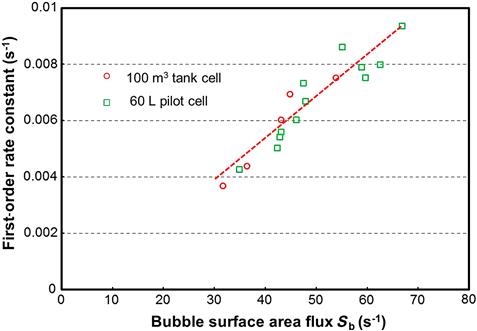
There is support for Eq. (12.29) taking a first principles approach to bubble–particle interaction (Finch, 1998), but the relationship is largely empirical.
Particles
The relationship expressed in Figure 12.33 introduces a new engineering measure of floatability, the proportionality constant P, a dimensionless quantity if kp and Sb are in expressed in the same reciprocal time units (e.g., s−1 as in Figure 12.33). The value of P is a reflection of particle properties: size, composition (liberation), and hydrophobicity. While treated as a constant, P is likely an inverse function of bubble size (Yoon, 1993; Hernandez-Aguilar, 2011); nevertheless the model (Eq. (12.29)) represents an advance over using the rate constant alone in analyzing flotation systems. Based on these findings, flotation performance can be considered to arise from the interaction of a stream property—the particle floatability (P)—with parameters that characterize the operating conditions of the pulp (Sb).
Making the analogy of the bubble/particle reaction to a chemical reaction means the derived kinetic model applies to the pulp (or slurry) zone, not to the overall cell, which includes froth.
Froth
Equation (2.29) can be modified by introducing a froth zone recovery factor. Figure 12.34 shows the concept of two interacting zones, pulp and froth, with dropback (1 − Rf) considered to be combined with the fresh feed to the cell (Finch and Dobby, 1990). Letting the feed (dry) solids mass flowrate to the pulp zone be X and introducing Rp as pulp zone recovery and Rf as froth zone recovery, the resulting solids flowrates are as indicated on the figure. A mass balance across the dashed line block gives the incoming feed F and thus the overall flotation cell recovery Rfc as:
(12.30)
(12.31)

Substituting Eq. (12.28) into Eq. (12.31), the overall flotation rate constant (kfc) is given by:
(12.32)
and substituting Eq. (12.29) into Eq. (12.32) gives the expression relating the overall flotation cell rate constant to the three contributing factors: particles (ore), machine, and froth.
(12.33)
The fully mixed first-order kinetic model then becomes:
(12.34)
Techniques to quantify the froth recovery factor continue to be developed (e.g., Seaman et al., 2004; Yianatos et al., 2008; Rahman et al., 2012). However, most methods are either intrusive in the froth or subject to assumptions (e.g., no entrainment). A method initially developed for batch flotation cells by Feteris et al. (1987) was later modified by Vera et al. (1999) to determine Rf directly on industrial flotation cells. In this approach, froth zone recovery (Rf) is estimated by determining the cell recovery at a measured froth depth (hence giving the overall cell first order rate constant, kfc) relative to the cell recovery at no froth depth (and hence giving the pulp (collection) zone rate constant, kp). The cell recovery at no-froth depth cannot be measured directly, but can be estimated by extrapolation of results obtained at four or more froth depths (Amelunxen and Runge, 2014).
Froth zone recovery is related to froth stability. As was the case in characterizing frothers’ froth stabilizing function (Section 12.5.6), the problem is one of definition and measurement. The notion is that there is an optimum froth stability that will give the best performance from a flotation cell, for example, maximum recovery at given grade, or maximum grade at given recovery (Farrokhpay, 2011). A promising measure of froth stability is air recovery, the fraction of the air delivered to the cell that overflows as unburst bubbles. Air recovery α can be calculated using the following expression:
(12.35)
where Qg is the total air flowrate into the cell, ζ the GH in the froth zone (usually assumed to be 1), vf the overflowing froth velocity, h the froth height over the lip, and w the length of the lip where froth is overflowing. Froth velocity is measured by a camera monitoring the surface of the froth as it overflows using image processing software. A concern could be raised regarding propagation of error involved in calculation from several independent measurements (what is a typical error, e.g., 95% confidence interval, on α?) plus the fact that some air may leave with the cell tailings. Nevertheless, air recovery has been successfully used. By manipulating air rate to cells to operate at maximum (or peak) air recovery (PAR) improved bank performance was obtained, marking a new approach in flotation circuit control and optimization (Hadler and Cilliers, 2009; Hadler et al., 2010).
12.9.4 Testing the k–Sb Relationship
To test Eq. (12.29) it is important not only to minimize the impact of froth (i.e., using shallow froth where Rf ~ 1) but also to ensure that two other considerations apply: that the pulp zone is operating in a “safe” range, and that the conditions approximate those of first order kinetics. A safe operating range refers to the air being adequately dispersed into bubbles. Yianatos and Henriquez (2007) suggest the following “safe” conditions: air velocity Jg 1–2 cm s−1, D32 1–1.5 mm and corresponding Sb 50–100 s−1. The reason there is a safe operating range is because the pulp cannot hold more than a certain volume of air. The volume of air is measured as GH (or εg), the volume of air divided by the total volume of slurry and air in the pulp zone (see Section 12.14.2). From observation, the maximum GH in mechanical cells and columns is about 15% (Finch and Dobby, 1990; Dahlke et al., 2005). If air rate is increased beyond that giving the maximum GH of ca. 15% it can result in loss of the pulp/froth interface and formation of large bubbles which disturb the froth, giving the appearance of boiling.
Operating in the safe range is a practical issue. The second consideration is a fundamental one: that conditions approach those for first-order kinetics. In writing Eq. (12.22) it was assumed that bubble surface area was not a restriction, that there was always space on bubbles to collect more particles. This assumption is approached when the concentration of floatable particles in the pulp is low. The first cells in a bank, especially a cleaner bank with a high feed concentration of floatable particles, will often violate the assumption; the froth overflow solids rate from the cell is now likely determined by bubble carrying capacity, the maximum mass of particles that can be transported to the overflow by the bubbles (Finch and Dobby, 1990). Based on the overflow cell area typical carrying capacity is ca. 1 t h−1 m−2 (Patwardhan and Honaker, 2000).
Respecting these restrictions then a linear k–Sb is supported (Hernandez-Aguilar et al., 2005); otherwise, a linear k–Sb relationship may not be observed, the rate constant could be independent of Sb or even decrease as Sb increases. Following the interpretation of Barbian et al. (2003), these deviations from linearity can be understood qualitatively by considering the way the particle load on the bubble changes as Sb is increased and the resulting effect on the froth: at low Sb the particle load per bubble will be high, perhaps giving too stable a froth, which does not flow readily; at a particular Sb the particle load may give an optimum froth stability; and at high Sb particle load may become too low to give adequate froth stability and froth overflow rate decreases. As froth zone recovery changes, so does the cell recovery and the derived overall rate constant.
While the importance of the froth to overall cell recovery is recognized it remains that the froth cannot deliver more mass than is delivered from the pulp. Some new cell designs aim to increase the pulp collection kinetics.
12.9.5 Modifications to Apply to Reactor–Separator Cell Designs (See Section 12.13.3)
The fully mixed kinetic flotation model expressed in Eq. (12.34) has been used primarily in analysis of mechanical cells and flotation columns. Some of the newer cell designs aimed at increasing the flotation rate fall into a category that can be described as “reactor–separator” designs. A feature of the reactor part is a high concentration of bubbles. In mechanical cells and columns, as noted, the volume fraction of gas that can be held in the pulp (GH) is limited to about 15%. In the reactor part of the reactor–separator cell designs GH can exceed 15%. For example, in the Jameson cell downcomer (the “reactor”) GH can approach 60% by having the slurry and air move concurrently (Marchese et al., 1992). In addition, in these reactors the energy input goes more directly into bubble–particle collision and attachment, rather than some energy being used to circulate pulp as in mechanical cells. In recognition, the pulp flotation rate constant in Eq. (12.29) can be modified to (Williams and Crane, 1983):
(12.36)
where Pg retains similar meaning (a factor associate with particle floatability, but based on GH rather than BSAF), and E is the energy directed to collision/attachment events. In consequence of the high bubble concentration, these new cell designs have much shorter retention times compared to mechanical cells and columns. For example, Harbort et al. (2003) report retention times in a Jameson cell circuit about 2–10 times shorter than in a mechanical cell circuit on the same duty; or up to one order of magnitude higher rate constant.
There is empirical support for Eq. (12.36). Hernández et al. (2003) reported a linear dependence of rate constant on GH in tests on flotation columns. Fundamentally, there is a question whether flotation rate depends on BSAF or GH. As noted in Section 12.5, from GH and bubble size the specific bubble surface area, Ab (bubble surface area per unit volume of gas), is given by Eq. (12.8):
(12.8)
This gives another modification to Eq. (12.29), namely:
(12.37)
where, again, Pa retains the meaning of floatabilty but now based on bubble specific surface area. Hence, kp is either dependent on the bubble surface area passing through the cell (Sb) or the bubble surface area in the cell (Ab), a potentially important distinction, but one not resolved.
Parameters corresponding to Sb and Ab are also associated with the particles; there is a particle surface area flux passing through the cell and a particle specific surface area in the cell. Part of the science of flotation is matching these particle and bubble parameters to optimize the process, tied up in the recurring question of what is the appropriate bubble size for a given particle size that resists an easy answer but is an ambition of fundamental modeling efforts (e.g., Bloom and Heindel, 2002).
From a practical perspective, in mechanical and column cells BSAF and GH are related, for example, both increase with an increase in air rate and a decrease in bubble size (Finch et al., 2000), so whether one or the other is “fundamental” could be considered moot. Compared to BSAF, from a measurement standpoint GH has the advantage as commercial GH sensors are available (CiDRA Minerals Processing). At least one plant has used online measurement of GH in developing column flotation control strategies (Amelunxen and Rothman, 2009).
12.10 The Role of Particle Size and Liberation
12.10.1 True Flotation
As with all mineral separation processes, recovery in flotation is particle size dependent (Chapter 1). The role of particle size is less pronounced compared to, say, gravity concentration, but analysis of recovery-by-size data can reveal opportunities for process improvement (Grano et al., 2014). With increased availability of liberation data, analysis of recovery-by-size-by-liberation data is adding an extra level of what can be called diagnostic metallurgy. Recovery-by-size is calculated from:
(12.38)
where Ri,m is recovery of mineral m of size i, C/F the mass fraction reporting to concentrate, ci, fi the mass fraction in size interval i in concentrate and feed, and ci,m, fi,m the assay of mineral m in size interval i in concentrate and feed. Data collection, therefore, requires sampling the process, sizing the samples, and assaying the sized fractions. There are the inevitable associated errors requiring data reconciliation to obtain useful information (Chapter 3).
Figure 12.35 shows a typical evolution of the recovery–size relationship as flotation time is increased. The figure reveals three size classes: an intermediate size range where recovery is high; a fine size range where recovery is lower and increases with time; and a coarse size range where recovery is again lower but less affected by time. The size divisions are not precise and will vary with mineral type. The data can be reexpressed as a rate constant versus size relationship (Figure 12.36).


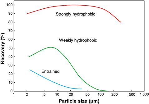
Figure 12.37 illustrates three types of recovery–size relationships: one for strongly floatable mineral, a second for weakly floatable mineral, and a third for mineral recovered by entrainment. For the strongly floatable mineral there is a broad intermediate size range of high recovery, while the less floatable mineral has a similar but size-compressed relationship. Any selective flotation process will see this combination of strong and weak floatable minerals, for example, selective flotation of base metal sulfides from each other and from pyrite.
Fine Particles
Particle recovery by true flotation involves collision, attachment and formation of stable attachment to bubbles, often expressed as probabilities (or efficiencies). Collision probability is governed by the physics of the process (or “hydrodynamics”), while attachment probability and stability of attachment include a chemical component (particle hydrophobicity). The decline in recovery at the fine end is usually ascribed to low collision probability, fine particles having insufficient inertia to cross the water streamlines around the coursing bubble. Note this does not say there is a lower particle size limit to flotation, only that the rate of flotation will decrease as particle size decreases. Figure 12.36 reinforces this conclusion, showing the fines have a low but finite rate constant. (Pease et al. (2006) make the point quite forcefully that there is not a lower size limit to flotation, just slowing kinetics.)
The collision-limited explanation of low recovery of fines implies that fine particles will be strongly influenced by flotation time, which is supported in Figure 12.35, and perhaps less affected by reagent additions that alter hydrophobicity, which can be the case (Trahar, 1981; Senior et al., 1994). Chemistry is not completely absent of course: fines are subject to surface oxidation and other contamination effects (e.g., adsorption of metal ions), and fines can cause aggregation (slime coating), issues that do respond to chemistry (Grano et al., 2014).
Increasing the rate of flotation of fine particles has obvious practical benefits. The requirement is to increase exposure to bubbles in order to provide more collision events and bubble surface area to transport collected particles. In an individual cell, increasing air rate and decreasing bubble size appear to offer means to achieve this increased exposure, the combination increasing Sb (Eq. (12.7)), which predicts an increase in rate constant (and the effect may be even greater than Eq. (12.7) predicts if P is inversely related to bubble size (Yoon, 1993)). Improved fine Pt-mineral recovery by frother addition to decrease bubble size is an example of successful implementation of this approach (Hernandez-Aguilar et al., 2006).
Increasing air or decreasing bubble size, however, also increases GH and there is this noted limit, about 15%, before a cell “boils.” The options to increase kinetics using air rate and bubble size in a cell are, therefore, limited. The practical option to increasing exposure to bubbles is to float for longer. In the laboratory the effect of time on increasing fine particle recovery is easy to demonstrate (Figure 12.35); in the plant, surveying cells cumulatively down a flotation bank will show the impact of increasing number of cells (i.e., time) on increasing recovery of fines (Trahar, 1981; Grano et al., 2014). The installed flotation capacity is often dictated by the slow floating fine particles, including the use of a scavenger stage to provide increased flotation time.
Rather than relying on increased exposure, the energy of interaction with the bubble could be increased to “force” the particles across the water streamlines to intercept the bubble. The positive effect of increasing energy input on fines flotation is known, which recent work using a specially designed cell to give uniform distribution of energy throughout the pulp has reinforced (Safari et al., 2013). Increased energy input can be achieved by increasing impeller speed in mechanical cells; an option sometimes exercised to increase fines recovery is to increase impeller speed down a bank of cells. The reactor–separator flotation cells aim to inject this energy more directly to the collection of fine particles, as noted in Eq. (12.36).
Coarse Particles
At the coarse end of the particle size spectrum, the decline in recovery probably includes a contribution from decreased liberation, but in terms of bubble–particle interaction events is usually attributed to decreased stability of attachment, that is, increased probability of detachment (Jameson, 2012). Dissipation of energy as fluid eddies causes the bubble–particle aggregate, such as depicted in Figure 12.1, to spin and the centrifugal force can dislodge the particle. Another factor is higher froth dropback of coarse particles (Finch and Dobby, 1990; Rahman et al., 2012). Detachment of the particle and froth dropback introduce a chemical aspect: addition of collector to increase hydrophobicity (increase contact angle in Figure 12.2) should increase stability of the bubble–particle aggregate in the pulp zone and particle retention in the froth zone and thus increase recovery. The positive impact of chemistry on the recovery of coarse particles is seen in the recovery–size data of Trahar (1981) and Senior et al. (1994). Loss of free coarse particles to tailings may indicate that altered chemistry is required.
In contrast to fine particles, high energy input is evidently detrimental to coarse particle recovery, as Safari et al. (2013) illustrate. To accommodate the different needs of fine and coarse particles some strategies have been implemented. Distributing collector along the bank is one (Bazin and Proulx, 2001). Low collector concentration at the head of the bank is sufficient for the fast floating intermediate-size particles and upon their removal further collector dosage down the bank can target recovering the slower floating coarse particles. Classifying feed into fine and coarse fractions is often discussed but there are few examples. At the Mt Keith operation the feed was first split into two size fractions then into three (Senior and Thomas, 2005), and the improved Ni recovery paid for the project within a month. The authors emphasized the benefits of understanding particle size effects. New cells combining teeter bed (hindered settling) and flotation principles are aimed expressly at enhancing coarse particle recovery (see Section 12.13.4).
The trend in the recovery vs. size shown in Figure 12.35 is qualitatively explained by the product of collision probability (that increases as particle size increases) and detachment probability (that decreases as particle size increases).
Liberation
Recovery-by-size-by-liberation data are not common, a situation set to change with the increasing spread of automated mineralogy technology (Chapter 17). A set of such data is given by Welsby et al. (2010), where liberation is considered to be surface liberation. Derived from their data, Figure 12.38(a) shows rate constant as a function of size and liberation. Figure 12.38(b) replots the data as rate constant relative to the maximum rate constant, k/kmax showing there is consistency to the rate constant–size relationship independent of liberation. Jameson (2012) noted this consistency in the data, showing the rate constant of liberation class kx relative to the rate constant of fully liberated mineral, klib (L=kx/klib), was a unique function of liberation (surface exposure, x) independent of particle size, that is, L=fn(x), introduced as a liberation function.

In predicting the rate constant for locked (composite) particles, a first approximation is that the rate constant of the liberation class kl is a weighted average (Nesset, 2011); for example, for a particle with three surface exposed minerals, A, B, and C the kl is given by:
(12.39)
where x is fractional surface exposure and k refers to rate constant of liberated mineral. From Eq. (12.39), a refinement of the liberation function might be to consider locked particle type, binary locked A, B particles as distinct from binary locked A, C particles, etc.
Recovery-size-liberation data offer the promise to interface comminution and flotation models (and other separation process models). The comminution step produces the size-liberation spectrum and the associated recovery (or rate constant) data for a separation unit can be used to predict the outcome (grade and recovery) from that unit. The common simplification is to assume that recovery–size data are independent of the size distribution of the feed to the separation unit and how the size distribution was produced. This simplified approach to interfacing comminution with flotation has been used over the years (Ramirez-Castro and Finch, 1980; Bazin et al., 1994; Bradshaw and Vos, 2013). A related assumption is that the size-liberation data are also independent of how the size distribution is generated. With the consistency evident in the rate constant-size-liberation relationship (Figure 12.38(b)), a way to include liberation in interfacing comminution and flotation may be forthcoming.
12.10.2 Entrainment
To increase fine particle recovery, increasing flotation time is the practical option. Increasing time incurs a penalty, however: increased entrainment recovery. The recovery–size relationship for entrained material (Figure 12.37), shows a trend distinct from the two floatable minerals, recovery increasing as particle size decreases especially below about 50 μm (Smith and Warren, 1989). Recovery of entrained particles is related to water recovery (Jowett, 1966). Water is transported by bubbles into and through the froth, and since particles are in the water (i.e., it is slurry that is actually carried by the bubbles), there is an unselective particle recovery mechanism. Entrainment recovery is a fine particle recovery mechanism as fines do not settle out of the transported water under gravity as fast as coarse particles. Johnson (1972), from industrial and lab-scale tests, established that recovery by entrainment was proportional to feed water recovery to the concentrate. From this finding the degree of entrainment was defined as the ratio of the recovery of entrained solids to the recovery of water Ci or ENTi where subscript i refers to a particular particle class (particle type and size). An estimate of dependence on size is shown in Figure 12.39, taken from Johnson (2010), who reviewed practical aspects of entrainment.

The dependence of entrainment on water transport has driven the need to understand (model) water recovery mechanisms. Several water recovery models were compared by Zheng et al. (2006). A physics-based simulator, FrothSim, was successfully used to model entrainment in assessing ways of controlling bank performance (Smith et al., 2008).
From an operations viewpoint, the dependence means that reducing entrainment requires reducing water recovery. There are several options.
Role of Cleaner
The rougher stage contributes the initial (and often large) entrainment and the cleaners play an important role in reducing it. Figure 12.40 illustrates an example of the cleaner’s effect on recovery-by-size for a floatable mineral (sphalerite) and entrained mineral (NSG). The rougher inputs significant entrained fine (<10 μm) NSG, which the combination of cleaner stages (or cleaner block) rejects (and at the same time the scavenger increases fine sphalerite recovery due to increased retention time, as discussed above). Cleaners do not fully eliminate entrainment; even after several stages of flotation there is evidence that operational changes can still be effective in reducing its impact (Cooper et al., 2004).

This role of cleaners in rejecting entrainment is one argument against by-passing products direct to concentrate. Candidate products include concentrates from the first cell in the rougher bank, a unit cell ahead of the roughers or a flash flotation stage inside the grinding circuit. These products might be “high grade” (e.g., exceeding final concentrate grade) but can still carry substantial entrained (−50 μm) material that would be easily rejected in a cleaner stage with little loss of value recovery. Not cleaning these products means the remaining feed to the cleaners has to be upgraded sufficiently to compensate, which is not always achievable.
Pulp Dilution
Increasing pulp dilution reduces water recovery (Johnson and Munro, 2002). It may seem counter-intuitive, but recall that water transport is via the bubbles. Diluting the feed to a flotation stage means increasing the feed rate of water, but since the bubbling rate is not changed (Sb is unchanged) then the rate of water carried to the concentrate does not change, at least to a first approximation. Since water recovery is the ratio of the concentrate water rate to feed water rate, the recovery goes down. Not necessarily practical in the roughing stage because of the volumes involved, pulp dilution to cleaner stages is widely practiced.
An illustration of the merit of cleaner feed dilution is described by Shannon et al. (1993). In that example dilution enabled the operation to take full advantage of increased liberation through regrinding by controlling entrainment of the additional fines produced. A reassignment of cleaner cell capacity retained the necessary retention time. Retrofitting pulp dilution while retaining the required retention time (e.g., by reassignment of cells) may not always be feasible and it is best to plan pulp dilution at the plant design stage.
Particles tend to stabilize froths and increase water recovery. This is one reason why flotation usually aims to float the mineral in least amount in the feed, to reduce entrainment (and entrapment) of unwanted minerals. Commonly the mineral in least amount is the valuable mineral and is floated, but in some cases such as processing iron ores, the gangue (silica) is in lesser amount and reverse flotation is practiced. In cleaner stages the floatable mineral becomes the majority and sometimes reverse flotation, for example, pyrite from base metal concentrates, is worth considering.
Air Rate
Knowing water transport is via bubbles introduces manipulating air rate to control entrainment. Cooper et al. (2004) found by lowering air rate in the first cells of a Zn-cleaner bank (and increasing air rate down the bank to maintain Zn recovery) improved the grade of bank concentrate. The improvement was attributed to decreased entrainment of NSG in the first cells due to the lower air rate.
Froth Depth and Wash Water
Increasing froth depth is a direct way to reduce entrainment and manipulation of froth depth is a common grade control strategy. Deep froths with wash water addition to control entrainment was probably the prime advantage of flotation columns when these units reemerged in the 1980s (Finch and Dobby, 1990). Wash water is added into the froth to replace the water coming from the pulp and thus eliminates the entrained particles coming with the pulp water. By replacing the water draining from the froth under gravity, the addition of wash water enables deep froths to be built. Entrainment control using wash water is successful on mechanical cells as well (Kaya et al., 1990).
Since reducing water consumption is a concern in most locations, wash water use is under some scrutiny. How to introduce wash water to minimize use while achieving the benefits remains a challenge (Neethling et al., 2006). Most operations appear to favor introducing wash water from over-head drip pans rather than submerged devices in order to facilitate visual checks. An example wash water addition system is shown in Section 12.13.2.
12.11 Cells, Banks, and Circuits
The purpose of this section is to provide a theoretical framework for the progression from single cells to banks to circuits that characterizes flotation plants. The emphasis is the effect on recovery and separation between floatable minerals (often referred to as “selectivity”).
12.11.1 Single Cell
Recovery
Introduced in Section 12.9, recovery in a single cell has two mathematical extremes depending on material transport, namely plug flow (Eq. (12.27)) and fully mixed flow (Eq. (12.28)).
For mechanical cells and flotation columns the fully mixed approximation is usually adopted. Figure 12.41 compares recovery as a function of kτ for the plug flow and fully mixed cases: it is evident, since k is the same for both, that more time is needed in a fully mixed cell to achieve the same recovery as under plug flow. For example, for a target recovery of 90% (0.9) the fully mixed kτ is 9 (solving Eq. (12.28), see Figure 12.41) and for plug flow kt is 2.3 (Eq. (12.27)). This means retention time is 9/2.3 (i.e., 3.9) times longer in the fully mixed case compared to plug flow: for equivalent recovery this translates to 3.9 times the cell volume being required in the fully mixed case compared to plug flow.

This difference in recovery between fully mixed and plug flow transport is well understood, one consequence is the need to scale up lab determined flotation time (i.e., equivalent to plug flow) to the continuous (industrial) case. A common scale up factor is 2.5 to estimate plant flotation time in sizing cells (Wood, 2002). (Increasing flotation time by 2.5 is equivalent to scaling down the rate constant by 2.5, noting that it is always the product kτ in the formulae.) Less realized perhaps is the impact of mixing degree on separation (selectivity) of floatable minerals.
Selectivity
To illustrate the impact of mixing on separation, consider two minerals A and B with rate constant kA=1 min−1 and kB=0.1 min−1 and take as the measure of efficiency the difference in recovery, that is, SE=RA – RB (Eq. (1.2)). Solving Eqs. (12.27) and (12.28) for these k values, we find that SE in the fully mixed case is 43% (0.43) and in the plug flow case SE is 69% (0.69) (Table 12.6). The lower selectivity in the fully mixed case can be seen in Figure 12.41; the slope is the rate of change in R with kτ (i.e., δR/δkτ) and it is evident that slope is higher for the plug flow case, meaning greater selectivity compared to the fully mixed case. (A convenient reference point is to compare δR/δkτ at R=0.5.) In summary, therefore, not only is more time (i.e., more cell volume) required in the fully mixed case to reach the same recovery as in plug flow but the SE is also less.
Table 12.6
Comparison of SE for Fully Mixed and Plug Flow Transport at Equal Target Recovery of Mineral A=90% (0.90) where kA=1 min−1 and kB=0.1 min−1
| Fully Mixed | Plug Flow | ||||||
| τ (min) | RA | RB | SE | t (min) | RA | RB | SE |
| 9 | 0.90 | 0.47 | 0.43 | 2.3 | 0.90 | 0.21 | 0.69 |

The analysis of selectivity can be addressed by writing Eq. (12.28) for both A and B and combining to eliminate τ (which is clearly the same for both minerals) to express RB as a function of RA. For the fully mixed case the result is:
(12.40)
 (12.40)
Introducing S as the relative rate constant (kA/kB) Eq. (12.40) becomes:
(12.41)
 (12.41)
Figure 12.42 shows the trend in RB with RA for S varying from “difficult” separation (S=2) to “easy” separation (S=10, equivalent to the situation above where kA=1 and kB=0.1). An example of a difficult separation is sphalerite from pyrite, where Cooper et al. (2004) reported S ~ 2–3. The figure shows the increasing rate of recovery of B with respect to A as recovery of A is increased.

Instead of expressing S as a relative rate constant, we could express in terms of relative floatability by expanding S in terms of the k–Sb relationship (Eq. (12.33)):
(12.42)
Since Sb is the same for both minerals and there is evidence that RfA=RfB for floatable minerals (Vera et al., 1999) then S ~ PA/PB.
Using SE and relative floatability, S, the following optimization problem can be addressed: to maximize SE (maximize selectivity) at target recovery. This optimization problem can be stated as follows:
Maximize
(12.43)
by searching on RA subject to
(12.44)
and
(12.41)
 (12.41)
Maximizing SE is equivalent to minimizing RB at the target RA or maximizing grade (specifically grade of A relative to B).
Applying to a single cell it is evident that the optimization problem cannot be solved: in a single cell it is not possible to satisfy two constraints, maximum SE and target RA (Maldonado et al., 2011).
Three limitations of the single fully mixed cell are therefore identified: the need for increased flotation residence time (i.e., cell volume) to attain the same recovery as in plug flow; the lower selectivity between floatable minerals compared to plug flow; and the inability to maximize SE at a target recovery. These limitations are addressed by placing cells in series; that is, to form a bank (or line or row).
12.11.2 Banks
Recovery
The calculation of bank recovery from individual cell recoveries is illustrated in Figure 12.43. Taking mass feed rate to the bank of unity (F=1) as a basis, the mass flows around each cell are calculated based on the cell recovery (relative to the feed to that cell). In Figure 12.43(a) the mass flows are shown for three cells; and in Figure 12.43(b) the general solution for N cells is given for the case where all cell recoveries are equal, Ri. The bank (total) recovery Rbk is given by the summation of the individual cell mass flows (since F=1, the mass flows are equivalent to fractional recoveries). In case (b) where all cells have equal recovery (Ri) the bank recovery can be derived directly from a mass balance around the dashed block:
(12.45)

Assuming equal cell recovery might seem a mathematical contrivance to provide a simple solution, but a justification for equal recoveries will be given when selectivity is considered. By substituting Eq. (12.28) into Eq. (12.45) and, noting that τi=T/N where T is the total bank retention time, the following is derived:
(12.46)
Figure 12.44 illustrates the impact of N: increasing N from 1 to 4 gives a significant increase in recovery for a given kT; in the limit as N → ∞, Eq. (12.46) becomes the plug flow solution, Rbk=1 – exp(−kT). Recovery approaches the plug flow result as the number of cells is increased because transport approaches plug flow (Figure 12.45).


Banks clearly give an advantage in recovery over one large cell of equivalent total volume. A question that arises is: how many cells should the bank comprise?
The analysis above implicitly assumed the individual cells are isolated and there is no short circuiting or back mixing between cells. The modern circuit of tank cells approaches the assumption: in that case Figure 12.44 suggests a bank of four or five cells is sufficient. Some care in this interpretation is required, however. Eq. (12.46) derives from Eq. (12.45), where all cells have equal recovery, making this the basis of the calculations. Significant deviation from equal recovery invalidates the solution, potentially making the four to five cell bank too short. As a resolution, six to eight cells to a bank may offer a practical compromise (Wood, 2002). A caveat is that in practice cells are often paired in a bank and act as one unit and this may represent an effective reduction in number of cells in the bank. (Note that in some plants “bank” refers to this pairing of cells, the whole being a row or line.) With older trough style banks of cells the impact of short circuiting between cells was countered by having long banks, up to 20 or more cells (Wood, 2002).
Figure 12.44 is a general solution independent of the magnitude of k: for example, if k is low this is compensated by selecting larger cells to increase T and maintain the kT value. In practice, longer banks (more cells) are usually recommended if k is considered low (Wood, 2002).
Short banks are encouraged by the increase in the size of mechanical cells, which over the past 50 years has gone from about 6 to 600 m3 (see Section 12.13.1). The advantage of large cells in reducing the number required and thus reducing capital and operating costs is an obvious incentive. To retain the recovery advantage of banks with large cells it is still necessary to keep a minimum number of cells in the bank, at least four, and preferably six to eight. The cost advantage of large cells is retained by reducing the number of parallel banks needed to reach plant throughput.
In constructing Figure 12.44 it was assumed that the retention time in each cell was the same, that is, each cell was the same volume. Maldonado et al. (2012) showed that for a given total bank capacity, cells of the same volume give the highest recovery; that is, equal size cells make best use of the installed volume. At the design stage there is little incentive to mix cell sizes, but there is less constraint in a plant expansion when a larger cell (usually at the head of the bank) can give the added volume perhaps more cheaply.
Selectivity
Gaining recovery for a given installed cell volume is one impact of the bank over a single cell. There is also a gain in separation between true floating minerals. Applying the optimization problem to a bank of cells, maximizing SE is solved by searching on RAi subject to the performance constraint (Eq. (12.44)) and the process constraint (Eq. (12.41)). Maldonado et al. (2011) illustrated the solution for two- and three-cell banks, which are amenable to trial-and-error solution, and went on to solve the general problem of an N-cell bank. The result is that the maximum in bank SE (SEbk, max) occurs when all cells have equal recovery, referred to as a balanced or flat bank recovery profile.
The physical interpretation derives from Eq. (12.41) and Figure 12.42. The relationship between RB and RA means that a cell recovering more A than its neighbor incurs a penalty of incremental B recovery that is not offset by another cell under-recovering A: if no cell should recover more than its neighbors then all cells must have the same recovery. There is evidence that this flat recovery profile does offer a metallurgical advantage over other profiles (Maldonado et al., 2012).
Figure 12.46 shows the impact of number of cells in the bank on SE: SEbk increases and levels off at about N=7 or 8. The physical interpretation is again based on Figure 12.42: increasing the number of cells means the recovery per cell is lowered which means the slope of the RB–RA relationship (δRB/δRA) is lowered; or in other words, less RB is recovered per RA recovery and thus selectivity is increased. There is evidently a potential loss in SE by having a bank shorter than about four cells, and, remember, the calculation in Figure 12.46 assumes the bank is operated with a flat recovery profile: a short bank with a nonflat profile risks even larger loss in SE than Figure 12.46 suggests. Again, we may have a practical compromise of six to eight cells in a bank. For older circuits with long banks, some up to 20 cells, balancing recovery is not really a concern; differences in recovery between so many cells will tend to be small and the profile will approach balanced.

The increase in SEbk as N is increased is reminiscent of the effect of N on recovery (Figure 12.44) and for the same reason: as N increases the bank approaches plug flow transport, which represents the theoretical maximum SE that can be achieved by the bank (Figure 12.46). Assuming plug flow for the bank and setting up the problem in the same fashion as in deriving Eq. (12.41), it can be shown that:
(12.47)
In the limit (plug flow) setting a target bank recovery of A determines the bank recovery of B for a known S and thus the maximum bank SE can be calculated.
Note that the analysis does not consider cell volume, only recovery. Having cells of different size complicates balancing cell recoveries, as a larger cell in the bank will naturally tend to recover more than its smaller neighbors. If plant expansion (or some other reason) suggests adding cells to a bank, the effect on selectivity, along with the noted effective use of cell volume in terms of recovery, is an argument in favor of the added cell having the same volume.
The optimization problem was to find a maximum in SE for a target bank recovery. We could extract the benefit in a different way: by setting a target SEbk the flat recovery profile will give the maximum bank recovery. The difficulty is knowing beforehand if the target SEbk is achievable.
Singh and Finch (2014), using JKSimFloat, explored two aspects not addressed in the analytical solution: variable S and impact of entrainment. The relative rate constant S will tend to decrease down the bank as high rate constant A particles are recovered in the first cells; in the example described they showed that this variation in S did not alter the flat recovery solution. Their examination of entrainment suggested the optimum operating condition was equal mass flowrate (mass pull) from each cell (flat mass pull profile), but that the flat recovery profile was close in performance. Entrainment is a significant factor in the roughing stage (e.g., Figure 12.40), perhaps less so in the cleaning stage when selectivity between floatable minerals is the focus. It is possible that different bank profiling strategies should be adopted for roughers and cleaners.
A review of standard texts does not reveal guidelines on bank operation. The flat recovery profile is offered as an operating strategy: the question then is how to achieve it. Some options discussed by Maldonado et al. (2012) are briefly reviewed.
Controlling a Flat Recovery Profile
Recovery profiling requires local cell control. One way, and the most rapid in response, is manipulation of air rate. Cooper et al. (2004) found using air to redistribute recovery down a Zn-cleaner bank gave improved performance (higher bank grade at target recovery). High recovery in the first cell of a bank is common because the high proportion of fast floating mineral renders recovery “easy.” Regardless of whether the flat recovery profile can be achieved, making sure the first cells do not “over-recover” is perhaps the principal practical outcome of the analysis. That observation holds whether maximizing selectivity or minimizing entrainment is the target; and is an argument that if a larger cell is to be added to a bank for some purpose that it not be made the first cell.
The Cooper et al. experience was on a cleaner bank where the first cells are probably carrying capacity limited rather than kinetically controlled. Nevertheless, there was an advantage to redistributing recovery down the bank suggesting that balancing recovery is a robust guideline.
Manipulating air rate down a bank became known as air rate (or Jg) profiling, part of a general strategy of air distribution management. An extension is PAR profiling (Hadler et al., 2012). In this strategy air rate to each cell in the bank is adjusted to achieve the maximum air recovery (Eq. (12.35)), which has been shown to maximize bank performance. Air distribution management to banks is gaining traction in flotation control strategies (Shean and Cilliers, 2011).
Online control of the recovery profile might be effected by monitoring froth velocity using froth imaging technology. If a relationship between froth velocity and recovery can be identified it would allow air to be manipulated to achieve the target froth velocity profile. As a first approach it may be easier to link froth velocity to mass pull rather than recovery, and consider the flat mass pull profile strategy identified by Singh and Finch (2014).
Variables other than air that might be considered for local cell control include froth depth (level), reagents, and impeller speed. Froth depth has been incorporated into air profiling (Gorain, 2005) and in the PAR strategy (Hadler et al., 2012). (In some control strategies froth depth is the principal manipulated local variable with air rate for fine tuning.) Distributing reagents along the bank and increasing impeller speed down the bank, both practiced to recover slow floating fractions (Section 12.10.1), have the effect of balancing recoveries. In general, reagents do not offer local control, as additions in one location will affect units downstream (and upstream through recycle). At one operation, reduced frother dosage was used to “slow down” the first cell in a bank when air rate could not be lowered sufficiently (Blonde et al., 2013).
12.11.3 Circuits
Compared to a single cell, the bank improves selectivity which approaches the theoretical maximum SE result for plug flow. A combination of flotation stages with recirculation, that is, a circuit (or network or flowsheet), enables the plug flow result to be exceeded. In general, a circuit will give better separation than single-stage operation, especially for nonsharp separations (Williams and Meloy, 2007), flotation being an example nonsharp separation system as the relative rate constant S imposes a limit to selectivity.
Selectivity
A basic circuit is shown in Figure 12.47, compromising two stages, the second being a scavenger to the first (i.e., treating the tailings from the first stage). This arrangement is familiar in the rougher–scavenger arrangement, and in the cleaner–cleaner/scavenger arrangement (the intended circuit depicted in the Figure). Circuit recovery can be solved by iteration, but also in an analogous fashion to that applied to Figure 12.34, this time introducing X as the mineral mass flowrate into the cleaner stage and deriving the (mineral) mass flows around the circuit (Figure 12.47). By mass balancing at the feed node (indicated by the circle), F can be deduced and the circuit recovery Rcirc solved:
(12.48)
(12.49)

The solution will be referred to as an “analytical” solution (an alternative name is “transfer function” (Williams and Meloy, 2007)). The impact of the circuit on SE can be judged by setting Rc and varying Rcs for the target mineral. Assuming the banks are long enough for plug flow to apply, the result for S=5 is shown in Figure 12.48(a). The calculation proceeds as follows: for A: select Rc,A (e.g., 0.2, 0.5, etc.), vary Rcs,A (e.g., from 0 to 1), calculate Rcirc,A using Eq. (12.49); and for B: from Rc,A and Rcs,A calculate Rc,B and Rcs,B using Eq. (12.47) with S=5, and solve for Rcirc,B using Eq. (12.49); finally, solve for SEcirc=Rcirc,A − Rcirc,B. The Figure shows circuit SE increases as Rcs increases. This increase in SEcirc is related to the increase in circulating load of A, given by:
(12.50)

The CLA is further increased by lowering Rc,A, as Eq. (12.50) indicates, and this further increases SEcirc as Figure 12.48(a) indicates. Putting all this together, Figure 12.48(b) shows the advance in SE going from single cell to bank (plug flow) to the two-stage circuit.
According to Figure 12.48(b), the circuit makes a significant increase in SE. This is indeed a circuit “property”, to improve selectivity. The magnitude of the impact shown, however, is exaggerated as the analysis implicitly assumed the recycled materials have the same recoverability as the fresh feed to the circuit. Figure 12.49, an example of rate constant versus size and liberation based on Figure 12.38(a), illustrates why this is not the case. The dashed horizontal lines indicate possible divisions for the cleaner and cleaner/scavenger stages; it is evident that the circulated material (CS con) comprises low rate constant material, namely fines, coarse and low grade (i.e., locked) particles. To take this variation in material properties into account requires simulators.

The analysis, nevertheless, does confirm why circuits are used in flotation: they increase selectivity between floatable particles (in addition to cleaners damping entrainment, Section 12.10.2). The benefit of the circuit, the circulating load, is also the “cost”: circulating loads mean increased stage (i.e., cell) volume is required. The target circulating load needs to be established at the design stage.
To optimize a circuit, Agar et al. (1980) suggested using the maximum SE at each stage. Based on Jowett (1975), they showed that the maximum in bank SE coincides with the cell in the bank that produces concentrate of grade equal to the feed grade; thus this cell defines the length of the bank. This is equivalent to selecting the length of bank such that no cell is yielding concentrate of lower grade than the feed to the bank, making it a tempting logical choice. However, using SE alone does not allow for the performance constraint of reaching a target recovery, nor does the strategy say how the bank is to be operated. It was later noted that maximizing stage SE does not result in maximizing circuit SE (Jowett and Sutherland, 1985; Lauder, 1992). The solution proposed here is to set the target circuit recovery of mineral A, then select the stage recoveries that meet that target and operate the stages with a balanced recovery profile. This will result in the maximum circuit SE at the target circuit recovery of A.
Varying target A recovery will generate the predicted relationship between SEcirc and Rcirc,A (such as Figure 12.48) to aid reaching a decision on where to operate (which could include an economic assessment) that will then give the corresponding stage recoveries. Repeating the calculations for the other mineral components (B, etc.) and summing gives total solids flows around the circuit and coupled with estimates of the water content (% solids) slurry volume flows can be calculated and stage cell volume requirements assessed. Agar and Kipkie (1978) used this approach, employing bench tests to determine stage recovery data for the mineral components (referred to as split factors) which were used to estimate the flow of mineral around a circuit by an iterative procedure. An example calculation using the analytical solution for the circuit in Figure 12.47 is included below (Example 12.1). The analytical approach helps understand the interactions between stages, which is further illustrated later. Once the circuit is decided, control of the circulating load is key to performance.
Example 12.1
For the circuit in Figure 12.47 calculate:
for the following conditions:
Mass flow (F)=100 t h−1; mineral feed grades fA=5% (0.05) and fB=95% (0.95).
Stage recoveries: RcA=0.75, RcB=0.10, RcsA=0.90, RcsB=0.15.
Solution
1. Mass flows.
From the mass balance:
this becomes the scaling factor to determine mass flows for any stream; note, for the individual minerals F=F f where f=fA of fB. The table below summarizes the calculations.
| Stream | Formula | Mass Flow (t h−1) | |
| A | B | ||
| Cleaner concentrate | 4.84 | 10.98 | |
| Cleaner tails | 1.61 | 98.84 | |
| Cleaner/scavenger concentrate (circulating load) | 1.45 | 14.83 | |
| Cleaner feed (as a check) | 6.45 | 109.83 | |

The cleaner feed calculation offers a check, where cleaner feed=fresh feed + circulating load:
For A: 6.45=5 + 1.45 (i.e., checks); and for B: 109.83=95 + 14.83 (i.e., checks).
2. Grades of and recoveries to cleaner concentrate.
From the table these are readily calculated:
While simplified, the calculation method offers a quick assessment, and for teaching purposes provides a calculation route that does not require a simulator to complete.
The arrangement in Figure 12.47 represents a component of a circuit. Some circuit options are considered.
Circuit Options
Table 12.7 shows some basic circuits. Simplifying by assuming equal recovery in each stage, the analytical solution for the circuit recovery can be found and is included in the Table. (To derive, a suitable starting point is required—e.g., in the R-S-C circuit letting X be feed to rougher, and in the R-C-CS circuit letting X be feed to the cleaner—and then proceeding as for Figure 12.47). Noble and Luttrell (2014) have considered over 30 circuits using this same basic approach.
Table 12.7
Some Common Circuit Arrangements, with Analytical Solution and Measure of Selectivity, the Slope (dRcirc/dR)
| Circuit | Circuit Recovery (all R Equal) | (dRcirc/dR) | |
| R-S-C |  |
||
| R-C-CS | 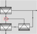 |
||
| R-C3-CS |  |
||
| R-S-C3 |  |
||
| (R-C-CS)2 |  |

The first two circuits in Table 12.7 represent the rougher–scavenger–cleaner circuit (R-S-C) and the rougher–cleaner–cleaner/scavenger circuit (R-C-CS). (In the first circuit it is traditional to refer to “scavenger” not rougher/scavenger.) The R-S-C circuit can be treated as the conventional arrangement providing as it does some buffering against the inevitable feed changes, enabling a level of manual supervision in preautomatic control days. The interaction between the stages, however, creates difficulties in control, as any action in one stage impacts the other stages. This made for a debate on advantages of open versus closed circuits (Lauder, 1992).
The R-C-CS circuit does partially open the circuit by isolating the rougher stage from the cleaner block (C-CS) with the CS tail being sent to final tail. The rougher function is now recovery (still at maximized SE) and the cleaner block function is grade. Independent control action appropriate to the two functions can then be implemented. In that regard the R-C-CS circuit is more “controllable” or “operable” than the R-S-C circuit. The stages may use different flotation machines, for example, flotation columns as the cleaner stage with mechanical cells in the cleaner/scavenger stage (Dobby, 2002).
It is common to regrind recycled material which will contain middling (composite) particles. Regrind is shown on the R-C-CS circuit (RG, which today would likely be a stirred mill) and could be included in the R-S-C circuit by combining the scavenger concentrate and cleaner tails. Regrind should always be considered. It may also permit a coarse primary grind if the mineral is readily floated, the lower mass of material making further grinding (regrinding) more energy efficient. Treatment of high tonnage porphyry copper ores often takes advantage of this approach.
Figure 12.50(a) compares Rcirc for the R-S-C and R-C-CS circuits as a function of R, the stage recovery. Two features are: (1) the Rcirc of the R-C-CS always lags that of the R-S-C and is less than the stage recovery (specifically the rougher stage) as there is no recycle to the rougher; and (2) the R-S-C circuit reduces recovery when R < 0.5 and enhances recovery when R > 0.5. This pivoting at R=0.5 points to how the R-S-C circuit increases SE, increasing the recovery of target mineral A with RA > 0.5 while decreasing the recovery of B with RB < 0.5. Selectivity is related to the slope of the Rcirc–R relationship, that is, (δRcirc/δR), and is included in Table 12.7 and plotted in Figure 12.50(b). Note that at high stage recovery (R > 0.7) the slope for R-C-CS circuit is greater than for R-S-C. This means that the selectivity between two minerals that have high and close recovery (i.e., low S) is greater in the R-C-CS circuit than in the R-S-C circuit. The R-C-CS circuit may not only be more “operable” but also offer an advantage in difficult selectivity cases, that is, ones with low relative rate constant, S. This general result is not altered by relaxing the assumption of equal stage recoveries, simply the magnitude of the SE changes (as illustrated in Figure 12.48).

This advantage of the R-C-CS circuit in difficult separation situations is more directly evident in Figure 12.51, which compares the SE of a single stage to that for the R-S-C and R-C-CS circuits under conditions of (a) “difficult” separation, S=2, and (b) “easy” separation, S=10. It is evident for the difficult case that at RA > 0.8 the R-C-CS circuit gives higher SEcirc than the R-S-C circuit. Since high recovery for the target mineral, i.e., high RA, is the target the R-C-CS circuit seems favored, the R-S-C circuit even failing to achieve the SE for a single stage at RA > 0.85. For easy separations (b), the R-S-C circuit seems the better choice; this would include when separation is primarily against entrained mineral, as in the case of recovering talc, coal, or bitumen.

In the late 1980s Brunswick Mine implemented the R-C-CS type circuit, with significant impact on Zn metallurgy, increasing the selectivity of sphalerite over pyrite (Shannon et al., 1993). This separation would be classed as difficult with S ~ 2–3 (Cooper et al., 2004). Sending CS tail to final tailings removed material that actually decreased performance if recycled to the rougher. Including regrind (ball mill/hydrocyclone) on the feed to the cleaner block (as in Table 12.7) to increase liberation, and diluting the pulp to control entrainment of the additional fines produced (Section 12.10.2) added to the advantage of the R-C-CS circuit. The circuit modification, which was a major simplification over the prior flowsheet, included removing a thickener. Thickeners do offer surge capacity and densification of feed to subsequent stages (regrind or flotation) but in some sulfide flotation circuits they may not be desirable by giving opportunity for oxidation and introducing a time lag that makes control difficult (Bulatovic et al., 1998). The modifications at Brunswick Mine were the start of an impressive series of improvements documented by Orford et al. (2005). During the 1990s the Noranda group moved to adopt the R-C-CS circuit across operations. The R-C-CS circuit is also common in Cu–Mo plants using columns as cleaners and mechanical cells as cleaner/scavengers (Bulatovic et al., 1998).
Opening the cleaner block by sending CS tails to final tails is not a decision taken lightly. Recirculating streams can appear to contain substantial mineral values but upon opening the circuit the flow diminishes and the amount of mineral lost to final tails represented by the CS tails is minor (and, as noted, trying to recover the contained values may be counter-productive). If there is concern over potential loss represented by the CS tails the stream could be considered for alternative treatments, upgrading by pyro- or hydrometallurgical processes, such as the Galvanox™ process (Dixon et al., 2007).
The next two circuits in Table 12.7 are developments on the first two. The R-C3-CS circuit introduces two additional cleaner stages to the R-C-CS network with cleaner 2 and cleaner 3 tails combined and recycled to the first cleaner via regrind. (Brunswick Mine had up to four cleaner stages in this arrangement.) The R-S-C3 circuit shows the conventional countercurrent flow arrangement. In the R-S-C3 circuit it is not easy to regrind all the recycled streams, which is a disadvantage. The analytical solution is also quite complex (to solve, incidentally, you have to start with feed to the last cleaner and work backwards through the circuit) compared to the solution for R-C3-CS, suggesting a strong interaction between stages, which makes for more difficult control. The number of stages could get quite large: prior to replacing with flotation columns the Cu–Mo separation circuit at Mines Gaspe had up to 14 countercurrent cleaning stages of mechanical cells (Finch and Dobby, 1990). Incidentally, rather than being referred to as cleaner 1, 2, etc. the cleaner stages may have local names, such as recleaner.
The last circuit supplements the basic R-C-CS circuit by repeating it, let’s call it (R-C-CS)2. This option allows for reagent additions into the second circuit aimed at the slow floating fractions. In that case the two concentrates will be combined. The same arrangement also serves when two minerals are to be recovered, for minerals A and B making the circuits (R-C-CS)A and (R-C-CS)B with separate concentrates.
Plants which concentrate two or more minerals may repeat circuits for each mineral or produce a bulk concentrate (e.g., a concentrate of at least two valuable minerals) then perform selective flotation on the bulk concentrate. Options are illustrated in Figure 12.52 for a Cu–Pb–Zn ore ranging from (a) “easy” milling ore where separate concentrates can be produced, to (b) more difficult ore where a bulk Cu–Pb concentrate is produced and then separated into Cu and Pb concentrates, to (c) where a bulk Zn–Pb concentrate is an additional final concentrate.

Circuit design is a combination of experience and increasingly the use of simulators, at least for the non-chemistry aspects (Herbst and Harris, 2007; Mendez et al., 2009; Ghobadi et al., 2011). While search algorithms may find optimal circuit configurations based on metallurgical performance criteria, in the end the choice has to be a circuit that is readily operated.
Circuit Flexibility
The decision having been reached to design a flotation circuit according to a certain scheme, it is necessary to provide for fluctuations in the flowrate and grade of ore to the plant.
The simplest way of smoothing out grade fluctuations and of providing a smooth flow to the flotation plant is by interposing a large agitated storage tank (agitator) between the grinding section and the flotation plant:
Any minor variations in grade and tonnage are smoothed out by the agitator, from which material is pumped at a controlled rate to the flotation plant. The agitator can also be used as a conditioning tank, reagents being fed directly into it. It is essential to precondition the pulp sufficiently with the reagents (including sometimes air, Section 12.8) before feeding to the flotation banks, otherwise the first few cells in the bank act as an extension of the conditioning system, and poor recoveries result.
Provision must be made to accommodate any major changes in flowrate that may occur; for example, grinding mills may have to be shut down for maintenance. This is achieved by splitting the feed into parallel banks of cells (Figure 12.53). Major reductions in flowrate below the design target can then be accommodated by shutting off the feed to the required number of banks. The optimum number of banks required will depend on the ease of control of the particular circuit. More flexibility is built into the circuit by increasing the number of banks, but the problems of controlling large numbers of banks must be taken into account. The move to very large unit processes, such as grinding mills, flotation machines, etc., in order to reduce costs and facilitate automatic control, has reduced the need for many parallel banks.

In designing each flotation bank, the number of cells required must be assessed: should a few large cells be incorporated or many small cells giving the same total capacity?
Some theoretical considerations have been introduced (Section 12.11.2), but there is a practical aspect as well: if a small cell in a bank containing many such cells has to be shut down, then its effect on production and efficiency is not as large as that of shutting down a large cell in a bank consisting of only a few such cells.
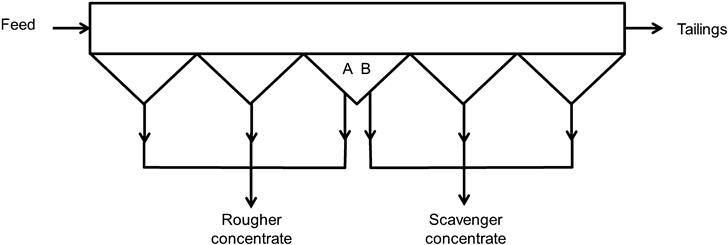
Flexibility can include having “extra” cells in a bank. It is often suggested that the last cell in the bank normally should not be producing much overflow, thus representing reserve capacity for any increase in flowrate or grade of bank feed. This reserve capacity would have to be factored in when selecting the length of the bank (number of cells) and how to operate it, for example, trying to take advantage of recovery or mass pull profiling. If the ore grade decreases, it may be necessary to reduce the number of cells producing rougher concentrate, in order to feed the cleaners with the required grade of material. A method of adjusting the “cell split” on a bank is shown in Figure 12.54. If the bank shown has, say, 20 cells (an old-style plant), each successive four cells feeding a common launder, then by plugging outlet B, 12 cells produce rougher concentrate, the remainder producing scavenger concentrate (assuming a R-S-C type circuit). Similarly, by plugging outlet A, only eight cells produce rougher concentrate, and by leaving both outlets free, a 10–10 cell split is produced. This approach is less attractive on the shorter modern banks. Older plants may also employ double launders, and by use of froth diverter trays cells can send concentrate to either launder, and hence direct concentrate to different parts of the flowsheet. An example is at the North Broken Hill concentrator (Watters and Sandy, 1983).
Rather than changing the number of cells, it may be possible to adjust air (or level) to compensate for changes in mass flowrate of floatable mineral to the bank. To maintain the bank profile at Brunswick Mine, total air to the bank was tied to incoming mass flowrate of floatable mineral so that changes would trigger changes in total air to the bank, while maintaining the air distribution profile (Cooper et al., 2004).
12.12 Flotation Testing
To develop a flotation circuit for a specific ore, preliminary laboratory testwork is undertaken to determine the choice of reagents and the size of plant for a given throughput as well as the flowsheet and peripheral data. Flotation testing is also carried out on ores and stream samples in existing plants to improve procedures and for development of new reagents.
Increasing attention is now paid to the need to understand variation in an orebody, and a procedure for the identification, sampling, and characterization of geometallurgical (geomet) units (or “domains”) has been successfully formulated and is now in common use (see Chapter 17).
Geometallurgical units (Lotter et al., 2003; Fragomeni et al, 2005) can be defined as an ore type or group of ore types that possess a unique set of textural and compositional properties from which it can be predicted they will have similar metallurgical performance. Sampling of an orebody based on geometallurgical units will define metallurgical variability and allow process engineers to design more robust flowsheet options. This variability can be muted when samples from different geometallurgical units are blended and tested as one sample. Rather, composite samples are created by ensuring grade and grade distributions from a specific area defining the geometallurgical unit within a resource are maintained. The method used to divide an orebody into geometallurgical units is based on a review of geological data including host rock, alteration, grain sizes, texture, structural geology, grade, mineralogy, and metal ratios with focus on characteristics that are known to affect metallurgical performance (Lotter et al., 2011). (The foregoing list is not complete and also includes hardness testing and the grade/recovery curve as characterizing parameters (e.g., Fragomeni et al., 2005).) Statistical analysis is often used to help define preliminary units. In addition, it is recommended that a variability program based on smaller samples taken from within and throughout a geometallurgical unit is completed prior to finalizing the divisions between geometallurgical units. This approach has a higher probability of capturing the full variance in composition and metallurgical behavior that can be expected from within a unit, and provides a cross check that the geometallurgical unit definition is robust.
Once a set of geomet units has been identified, sampled, and tested, the investigator is in a position to prepare a known composite using increments of each geomet unit to represent an overall plant mill feed mixture. At this point, the mixture may demonstrate interactions that either improve or deteriorate the metallurgical performance, so this last step is essential.
The purpose of sampling is to obtain an unbiased set of increments from the lot being sampled in such a manner that, when the increments are combined as a sample, the sample has the same composition as the lot that was sampled; the only difference is that the mass of the sample is less than the mass of the lot (Chapter 3). It is a definite recommendation that a proven, quantitative sampling protocol be used in the selection of increments to the sample to be used for flotation testing. In the procedure “High Confidence Flotation Testing” (Lotter, 1995a), use is made of the 50-piece experiment by Gy (1979) to obtain the sampling equation and associated minimum sample mass for a plant mill feed. This procedure is detailed elsewhere (Bartlett and Hawkins, 1987; Lotter, 1995b; Lotter et al., 2013); however, it is sufficient to remark that this approach plus use of Gy’s safety line to prepare the replicate batch test charges of ore negates any argument that the material brought to the test bench in the laboratory is not representative (Lotter and Oliveira, 2013; Lotter, 1995c; Lotter and Fragomeni, 2010). An alternative sampling method validated by Lotter and Oliveira (2011) uses drill core and drill core data to sample the population physically and mathematically so as to match the parent valuable metal distribution, and tests for agreement between the parent and sample distributions using the χ2 test (Lotter and Oliveira, 2013).
Having selected representative samples of the ore, it is necessary to prepare them for flotation testing, which involves comminution to the target particle size. Crushing must be carried out with care to avoid accidental contamination of the sample by grease or oil, or with other materials that have been previously crushed. (Even in a commercial plant, a small amount of grease or oil can temporarily upset the flotation circuit.) Samples are usually crushed with small jaw crushers or cone crushers to about 0.5 cm and then to about 1 mm with crushing rolls closed with a screen.
Storage of the crushed sample is important, since oxidation of the surfaces is to be avoided, especially with sulfide ores. Not only does oxidation inhibit collector adsorption, but it also facilitates the dissolution of heavy metal ions, which may interfere with the flotation process (Section 12.7). Sulfides should be tested as soon as possible after obtaining the sample and ore samples must be shipped in sealed drums in as coarse a state as possible. Samples should be crushed as needed during the testwork, although a better solution is to crush all the samples and to store them in an inert atmosphere.
Wet grinding of the samples should always be undertaken immediately prior to flotation testing to avoid oxidation of the liberated mineral surfaces. Batch laboratory grinding, using ball mills, produces a flotation feed with a wider size distribution than that obtained in continuous closed-circuit grinding; to minimize this, batch rod mills are often used which give products having a size distribution which approximates that obtained in closed-circuit ball mills. True simulation is never really achieved, however, as high-specific-gravity minerals in a plant grinding circuit are ground finer than the average due to recycling by the cyclone, which is a feature missed in a batch mill. It is also important to understand the effect of grinding media on flotation, making it sometimes difficult in the lab to simulate the plant chemical conditions (Section 12.8).
Predictions from laboratory tests can be improved if the mineral recovery from the batch tests is expressed as a function of mineral size rather than overall product size. The optimum mineral size can be determined and the overall size estimated to give the optimum grind size (Finch et al., 1979). This method assumes that the same fineness of the valuable mineral will give the same flotation results both from closed-circuit and batch grinding, irrespective of the differences in size distributions of the other minerals.
The potential for liberation of the minerals contained in the ore can be determined by characterizing the grain sizes of the minerals present (Chapter 17). This can be achieved by breaking the drill core samples at a relatively coarse size (typically about 600 µm) to preserve the in situ texture of the samples, including grain size, association, and shape. The texture can be characterized by using a scanning electron microscope configured as a mineral liberation analyzer, such as the MLA or the QEMSCAN (Chapter 17). Such an analyzer can measure the grain sizes and composition of the component minerals of the ore.
Testwork should then be carried out over a range of grinding sizes in conjunction with flotation tests in order to determine the optimum flotation feed size distribution. If the mineral is readily floatable a coarse grind may be utilized, and the subsequent concentrate regrinding to further liberate mineral before further flotation will mean a reduction in grinding costs per ton treated.
12.12.1 Small-Scale Tests
A measurement widely used in basic studies is the contact angle (Figure 12.2). The measurement can be made by attachment of a bubble on a polished surface of a mineral held in the solution (of collector, etc.) under test (“captive bubble” test). The contact angle on particles can be inferred from measuring pressure drop as a test solution is passed through a bed of particles. Most surface chemistry texts will describe the procedures. Some quasi-first principles flotation simulators use measured values of contact angle to predict grade/recovery. A related test is “bubble pick” where a bubble is exposed to particles in the test solution and the mass collected or angle subtended on the surface by the attached particles (the two are related) is measured (Chu et al., 2014).
There are a variety of devices designed to float about 1 g of mineral particles (e.g., Partridge and Smith, 1971; Bradshaw and O’Connor, 1996). In the Hallimond tube technique (Figure 12.55), the mineral particles (powder) are supported on sintered glass inside the tube containing the test solution. Air (or any other gas) bubbles are introduced through the sinter and any hydrophobic mineral particles are lifted by the bubbles, which burst at the water surface, allowing the particles to fall into the collecting tube. By treating a weighed sample of mineral, the weight collected in the tube can be related to the floatability. The technique can be adapted to simple mineral mixtures for some assessment of selectivity. The Hallimond tube has the advantage that assaying is largely avoided and the procedure is straightforward (sample preparation notwithstanding), however it is doubtful whether the method, especially as conducted on single minerals, simulates industrial flotation.

On a somewhat larger scale, the EMDEE Microflot Agitator uses up to 10 g samples (Chudacek, 1991). The device is a tube half filled with test solution and subjected to controlled agitation, which produces bubbles and partitions the particles between the pulp and the resulting froth. Tested on size fractions, the partitioning results were shown to correlate well with the rate constant determined by batch flotation tests. Bradshaw and Vos (2013) have refined the technique, retaining the testing of sized fractions to develop a Mineral Separability Indicator (JKMSI). By characterizing the size-by-size behavior it is possible to take advantage of the consistency of the recovery–size relationship (Section 12.10.1) in predicting full-scale results. A small scale test that simulates industrial flotation has obvious merit when limited samples are available.
12.12.2 Batch Flotation Tests
The bulk of laboratory testwork is carried out in batch flotation cells usually with 500 g, 1 kg, or 2 kg samples. The cells are usually mechanically agitated, the speed of rotation of the impellers being variable. A standard design is shown in Figure 12.56; variations aiming to improve reproducibility include bottom agitated cells and automated froth removal. Bottom-driven cells provide an unhindered surface which facilitates insertion of probes (pH, etc.).

In Figure 12.56 introduction of air is via a hollow standpipe surrounding the impeller shaft. The action of the impeller draws air down the standpipe, the flowrate being controlled by a valve and by the speed of the impeller; that is, the cell is self-aspirated. The setup can be adapted for controlled forced air addition. The air stream is sheared into fine bubbles by the impeller (discussed later, Section 12.13.1), these bubbles then rising through the pulp to the surface, where any particles picked up are removed as mineralized froth.
Batch tests are fairly straightforward, but a few points are worth noting (see also Wood (2002) and Runge (2010)):
1. Agitation of the pulp must be vigorous enough to keep all the solids in suspension, without breaking up the mineralized froth column.
2. Conditioning of the pulp with the reagents is often required. This is a period of agitation, varying from a few seconds to several minutes, before the air is turned on, which allows the surface of the mineral particles to react with the reagents.
3. Very small quantities of frother can have marked effects, and stage additions are often needed to control the volume of froth. The froth depth should be between 2 and 5 cm, as very shallow froths risk losing pulp into the concentrate container. Reduction in air rate is sometimes used to limit the amount of froth produced. This should be standardized for comparative tests to prevent the introduction of another variable.
4. Test should be at low pulp density (e.g., 10% solids) to avoid overloading bubbles (one reason being this invalidates conditions for first order kinetics). (As a matter of economics, industrial separations, at least at the roughing stage, are carried out in as dense a pulp as possible consistent with good selectivity and operating conditions. The denser the pulp, the less cell volume is required, and also less reagent is required, since the effectiveness of most reagents is a function of their concentration in solution. Most commercial rougher floats are in pulps of 25–40% solids by weight, although they can be as low as 8% and as high as 55%. In cleaner stages pulps may be diluted to take advantage of increased selectivity against entrained material (Section 12.10.2).) It must be borne in mind that in batch flotation tests the pulp density varies continuously, from beginning to end, as solids are removed with the froth and water is added to maintain the cell pulp level. This continuous variation changes the concentration of reagents as well as the character of the froth.
5. As water contains dissolved chemicals that may affect flotation, water from the supply which will be used commercially should be employed, rather than, say, distilled water. Any water added should contain some frother to maintain the bubble size in the pulp.
6. Normally only very small quantities of reagent are required for batch tests. In order to give accurate control of their addition rates, they may have to be diluted. Water-soluble reagents can be added as aqueous solutions by pipette, insoluble liquid reagents by graduated dropper or hypodermic needle. Solids may either be emulsified or dissolved in organic solvents, providing the latter do not affect flotation.
7. Recovery of froth is sensitive to operator technique, which is why automated froth removal methods are recommended.
8. Batch tests tend to produce significant entrainment recovery and allowance for this in determining kinetic parameters may be warranted (e.g., Ross, 1990).
9. Most commercial flotation operations include at least one cleaning stage, in which the froth product is refloated to increase its grade, the cleaner tailings often being recycled. Since cleaner tails are not recycled in batch tests, they do not always closely simulate commercial plants. If cleaning is critical, cycle tests (lock or locked cycle tests) may have to be undertaken.
Locked Cycle Tests
These are multiple-step flotation tests designed to measure the effect of circulating materials to provide a better insight into the expected performance from multistage processing of an ore. To incorporate the effect of recycle streams, the tests are performed multiple times with the recycled stream from a previous interaction added in the subsequent test. Normally at least six cycles are required before the circuit reaches equilibrium and a complete material balance should be made on each cycle. Since the reagents are in solution, it is essential that liquids as well as solids recirculate, so any liquid used to adjust pulp density must be circuit liquid obtained from decantation or filtration steps. Cycle tests are very laborious to carry out, and often the test fails to reach steady state. Procedures have been developed to simulate the locked cycle test steady state result from individual batch flotation test data (Agar and Kipkie, 1978; Runge, 2010).
Two other test procedures which use multiple flotation steps are release analysis (Dell, 1964) and tree flotation (Pratten et al., 1989). Devised to determine coal washability (i.e., the liberation-limited separation of coal from ash), they serve to show how close the actual operation is to the best possible performance. In establishing the effectiveness of new flotation machines, one way is to show the separation approximates the release or tree flotation result (e.g., Adel et al., 1991).
High-Confidence Flotation Testing
This method for has become a standard in some flotation laboratories (Lotter, 1995a,b; Lotter and Fragomeni, 2010). The approach is based on the following criteria:
1. The sample of ore presented to the flotation testing laboratory must be representative. This is achieved by use of Gy’s minimum sample mass and safety line models, combined with appropriate blending and subsampling protocols (Chapter 3).
2. Provided that the mass balance is maintained within certain limits across the flotation test, the built-up (or back-calculated) head grade should be in agreement with the sample mean grade of the assay heads within an acceptable error.
3. The use of replicate flotation tests assembled into composites, with the use of appropriate quality controls to reject outliers, instead of relying on single flotation tests for data, has a significant influence in reducing and normalizing the random errors.
The layout of the method is shown in Figure 12.57. Apart from its focus on representative sampling to produce reliable test material, which is shown as Section 1 in Figure 12.57, it has a structure of replicate flotation tests with associated quality controls that identify outlier tests and reject these at the 95% confidence level, as shown in Section 2 of the figure. The number of replicate tests required is dependent on the sample standard deviation that is typical of the ore type in question, and of the format of the flotation test. If the ore is unknown, it is best to perform a set of baseline rougher float tests and empirically obtain an estimate of the sample standard deviation.

The acceptable error in the table of 3.3% is based on experience with S. African Pt ores; the acceptable error needs to be established for the ore in question, using techniques introduced in Chapter 3.
Additionally, investigators should have a clear idea of the differences in grade and recovery that they may want to demonstrate (Napier-Munn, 2012). For base metal ores, triplicates are often suitable. However for precious metal bearing ores, or in cases where the ore is polymetallic bearing both base metal and precious metals, the number of replicates may be as high as five. In either case, the sample standard deviation and relative standard deviation (RSD) are calculated from these replicate tests for the first flotation concentrate mass. If this exceeds an RSD of 5%, the quality control triggers a check for outliers using the small data set model after Grubbs (1969). Outliers are then rejected, leaving the original set of replicate tests short.
Repeat flotation tests are then performed to replace the rejected outliers. Thereafter, acceptable replicates are taken into a set of composite concentrates and tailings for assaying and mass balancing. This amounts to the equivalent use of averages instead of singleton observations, a tenet of the Central Limit Theorem in statistics, which reduces overall random error and leaves any residual error distributed almost in the pattern of a normal distribution (Box et al., 2005). Use of this method puts the investigator in a position to compare smaller differences in grade and recovery between tests using different conditions, for example, reagent suite A versus B.
In Figure 12.57, the trial metal balance produces an independent estimate of the ore grade (the built-up head) from the weights and metal grades of the flotation test products. This built-up head value is compared to the sample mean assay head produced earlier in Section 1 of the model. The percent difference, using the assay head as the 100% basis, may trigger some repeat investigation of assays because of excessive error in the trial metal balance (i.e., in excess of ±3.3% in the case of Figure 12.57), calling for new subsamples of the assay heads and flotation test products (legend “1”). If this does not resolve the metal balance error, final resort activities indicated by legend “2” are triggered, calling for a new set of flotation tests.
The largest risk in any greenfield project is the scale-up from laboratory to operations at commissioning. The High Confidence Flotation Testing methodology has demonstrated accurate scale-up properties in the development and prediction of a flowsheet for a new orebody (Lotter and Fragomeni, 2010). For example, in the flowsheet development testwork for the Ivanhoe Kamoa copper project, which may be used as a relevant case study of this practice, the error in the copper metal balances averaged −0.3% with 80% of the individual errors falling between ±2% (Lotter et al., 2013).
Presenting Data
In addition to the common methods of presenting separation data, which include grade–recovery, recovery–mass recovery, and recovery–recovery plots (Runge, 2010), in flotation testing for scale-up time is also used a variable. Appendix VI gives a set of data on flotation of a Pb-ore collected as a function of time. The data can serve to illustrate all the data presentation methods, but here just time-based plots are presented, first to illustrate locating the maximum SE, following Agar et al. (1980) as introduced previously (Section 12.11.3), and second to estimate the flotation rate constant.
1. Maximum SE
This is located in two ways: at the time when the difference in recovery, in this case of galena versus the rest (lumped as one gangue G), is maximum; and at the time when the increment of grade is equal to the feed grade.
The computations (Appendix VI) involve determining cumulative recovery of Pb (galena) and gangue G. To determine the latter, the Pb assay has to be converted to galena mineral assay (see Example 1.1) with G determined by difference, 100−%galena. The resulting plot is shown in Figure 12.58. It is evident that the time when maximum SE occurs does correspond to the time when the increment in grade equals the feed grade. (Note that the increment of grade is plotted against the average of the time interval.) Translating to the case of a bank, it led to the notion that the optimum length of the bank would be that cell producing the same grade of concentrate as the feed (Section 12.11.3).
2. Determining flotation rate constant
In batch flotation the assumption of first order kinetics gives the following result (model) from Section 12.9.1:
(12.26)
It is important that the conditions do not change while performing the test, and this includes physical conditions such as air rate as well as chemical conditions. Figure 12.59(a) illustrates the “disappearance” plot (ln (1−R) vs. t), with slope k. Taking the data up to about 80% recovery gives k=0.88 min−1, which Figure 12.59(b) shows gives a reasonable fit to the recovery–time data.


Extending the disappearance plot to all the data, it is evident that a single k does not cover the full range (the reader should test this). To improve the fit has resulted in various modifications to the simple form of Eq. (12.26). Two modifications are: (1) introducing a maximum recovery less than 100% by rewriting as:
(12.51)
where R∞ refers to recovery after infinite flotation time; and (2) introducing the notion of fast and slow floating components:
(12.52)
where Øf refers to the fraction of fast floating mineral (the fraction of slow floating mineral is then (1 − Øf)), and subscripts f and s refer to fast and slow. This could be expanded to consider a nonfloating component as well. These refinements are referred to as a floatability component model (FCM).
There are any number of curve-fitting routines to estimate the parameters in these models, including Excel Solver. For example, the best-fit parameters for model Eq. (12.51) are R∞=97.62% and k=0.95 min−1. Plotting, however, remains a useful visual check.
What is being recognized in these modifications is that the rate constant has a distribution of values, which has led to attempts to describe this distribution with mathematical functions (Weiss, 1985). Klimpel (1980) assumed a rectangular distribution, which leads to the following solution:
(12.53)
where K is the maximum rate constant in the distribution. Klimpel made use of this model in plant evaluations by determining the effect of variables, for example, collector, on R∞ and K noting sometimes K would increase but R decrease and vice versa, the so-called “R–K trade-off.”
The distribution of k values derives from the effect of particle size and liberation illustrated in Figure 12.38; that is, it is “property based.” It would seem best to determine the rate constant on a size-liberation basis. This represents a large experimental effort for one condition and may become prohibitive if dependence on other conditions, for example, process chemistry, is to be considered. Welsby et al. (2010) show these property-based parameters can be related to floatability components—fast, slow, and nonfloating—and thus the simpler FCM can be used. Using an FCM, it should be possible to reassign floatability components following a change in feed stream properties (such as particle size), instead of rederiving them, a large reduction in experimental effort. It must be appreciated that data fitting exercises are accompanied by a degree of uncertainty in the derived parameters that can be high (Sandoval-Zambrano and Montes-Atenas, 2012). Simulations provide trends in metallurgy rather than precise predictions.
Cell Sizing (Example 12.2)
With the target retention time established, calculation of cell volume is relatively straightforward. Based on Wood (2002), the computation is as follows:
(12.54)