
Sampling, Control, and Mass Balancing
This chapter deals with the collection, analysis, and use of process data. Collection of reliable data is the science of sampling. The collected samples are analyzed for some quality, metal content (assay), particle size, etc. and the data are used for process control and metallurgical accounting.
Keywords
Sampling basics; sampling equipment; on-line analysis; process control; mass balancing; data reconciliation; example calculations
3.1 Introduction
This chapter deals with the collection, analysis, and use of process data. Collection of reliable data is the science of sampling. The collected samples are analyzed for some quality, metal content (assay), particle size, etc. and the data are used for process control and metallurgical accounting.
Computer control of mineral processing plants requires continuous measurement of such parameters. The development of real-time on-line sensors, such as flowmeters, density gauges, and chemical and particle size analyzers, has made important contributions to the rapid developments in this field since the early 1970s, as has the increasing availability and reliability of cheap microprocessors.
Metallurgical accounting is an essential requirement for all mineral processing operations. It is used to determine the distribution and grade of the values in the various products of a concentrator in order to assess the economic efficiency of the plant (Chapter 1). The same accounting methods are used in plant testing to make decisions about the operation. To execute metallurgical accounting requires mass balancing and data reconciliation techniques to enhance the integrity of the data.
3.2 Sampling
Sampling the process is often not given the consideration or level of effort that it deserves: in fact, the experience is that plants are often designed and built with inadequate planning for subsequent sampling, this in spite of the importance of the resulting data on metallurgical accounting, process control or plant testing and trials (Holmes, 1991, 2004). A simple example serves to illustrate the point. A typical porphyry copper concentrator may treat 100,000 tons of feed per day. The composite daily sub-sample of feed sent for assay will be of the order of 1 gram. This represents 1 part in 100 billion and it needs to be representative to within better than ±5%. This is no trivial task. Clearly the sampling protocol needs to produce samples that are as representative (free of bias, i.e., accurate) and with the required degree of precision (confidence limits) for an acceptable level of cost and effort. This is not straightforward as the particles to be sampled are not homogenous, and there are variations over time (or space) within the sampling stream as well. Sampling theory has its basis in probability, and a good knowledge of applied statistics and the sources of sampling error are required by those assigned the task of establishing and validating the sampling protocol.
3.2.1 Sampling Basics: What the Metallurgist Needs to Know
In order to understand the sources of error that may occur when sampling the process, reference will be made to probability theory and classical statistics—the Central Limit Theorem (CLT)—which form the basis for modern sampling theory. Additionally important to understanding the source of sampling error is the additive nature of variance, that is, that the total variance of a system of independent components is the sum of the individual variances of the components of that system. In other words, errors (standard deviation of measurements) do not cancel out; they are cumulative in terms of their variance. In general sampling terms this may be expressed as (Merks, 1985):
(3.1)
where ![]() , and
, and ![]() are the respective variances associated with error due to: i) heterogeneity among individual particles in the immediate vicinity of the sampling instrument, ii) variation in space (large volume being sampled) or over the time period being sampled, iii) the stages of preparation of a suitable sub-sample for analysis, and iv) the elemental or sizing analysis of the final sub-sample itself. This representation is convenient for most purposes, but total error may be subdivided even further, as addressed by Gy (1982), Pitard (1993), and Minnitt et al. (2007) with up to ten sources of individual sampling error identified. For the purposes of the discussion here, however, we will use the four sources identified above.
are the respective variances associated with error due to: i) heterogeneity among individual particles in the immediate vicinity of the sampling instrument, ii) variation in space (large volume being sampled) or over the time period being sampled, iii) the stages of preparation of a suitable sub-sample for analysis, and iv) the elemental or sizing analysis of the final sub-sample itself. This representation is convenient for most purposes, but total error may be subdivided even further, as addressed by Gy (1982), Pitard (1993), and Minnitt et al. (2007) with up to ten sources of individual sampling error identified. For the purposes of the discussion here, however, we will use the four sources identified above.
Some appropriate terminology aids in the discussion. The sampling unit is the entire population of particles being sampled in a given volume or over time; the sampling increment is that individual sample being taken at a point in time or space; a sample is made up of multiple sampling increments or can also be a generic term for any subset of the overall sampling unit; a sub-sample refers to a sample that has been divided into a smaller subset usually to facilitate processing at the next stage. It is important to recognize that the true value or mean of the sampling unit (i.e., entire population of particles) can never be known, there will always be some error associated with the samples obtained to estimate the true mean. This is because, as noted, the individual sampled particles are not homogeneous, that is, they vary in composition. This notion of a minimum variance that is always present is referred to as the fundamental sampling error. Good sampling protocol will be designed to minimize the overall sampling variance as defined in Eq. (3.1), in a sense, to get as close as practical to the fundamental sampling error which itself cannot be eliminated.
One of the pioneers of sampling theory was Visman (1972) who contributed a more useful version of Eq. (3.1):
(3.2)
where ![]() =variance: total, composition, distribution, preparation, and analysis; mi=mass of sample increment; n=number of sampling increments; and l=number of assays per sample.
=variance: total, composition, distribution, preparation, and analysis; mi=mass of sample increment; n=number of sampling increments; and l=number of assays per sample.
It is evident from Eq. (3.2) that the error associated with composition can be reduced by increasing both the mass and the number of sampling increments, that the error associated with distribution can be reduced by increasing the number of increments but not their mass; and that assay error can be reduced by increasing the number of assays per sample. We will now proceed to discuss each of the components of the overall sampling variance in more detail.
Composition Variance
Also known as composition heterogeneity, it is dependent on factors that relate to the individual particles collected in an increment, such as particle top size, size distribution, shape, density and proportion of mineral of interest, degree of liberation, and sample size, and is largely the basis for Pierre Gy’s well-known fundamental equations and Theory of Sampling (Gy, 1967, 1982). Gy’s equation for establishing the fundamental sampling error will be detailed later in this section. To illustrate the importance of relative mineral proportions in composition variance, consider a particle comprised of two components, p and q. The composition variance can be described as:
(3.3)
Figure 3.1 shows the composition variance as a function of mineral proportion p over the range 0 to 100%. Variance is at a maximum when the proportion of p in particles is at 50% and at a minimum as it approaches either 0% or 100%. Clearly, composition variance will be minimized the closer we get to individual mineral particle liberation. Achieving (at or near) liberation is therefore an important element of sampling protocols, particularly in the sub-sampling stages for coarser materials.

This is an important factor that needs to be understood about the system that is being sampled. The micrographs in Chapter 1 Figure 1.5 illustrate that various mineralogy textures will produce very different liberation sizes.
Selecting the appropriate sample size is also key to minimizing composition variance as noted in Eq. (3.2), and there are many examples of underestimating and overestimating precious metal content that can be traced back to sample sizes that were too small. Based on a computational simulation, the following two examples illustrate the problems associated with sample size (Example 3.1 and 3.2).
Example 3.1
Determine an appropriate sample size for mill feed (minus 12 mm) having a valuable mineral content of 50% (e.g., iron ore).
Solution
From the simulation, sample increment sizes ranging from 10 to 10,000 g were taken 100 times to generate statistical data that are free from the effect of sampling frequency. Table ex 3.1 and Figure ex 3.1-S illustrate that total error (expressed as relative standard deviation, σ, or coefficient of variation) reaches a limiting value of about 5% when the sample size is 5 kg or greater. In a sense, this value approaches the fundamental sampling error. The pitfall of selecting a sample size that is too small is clearly evident from the table and figure. Coarser materials require a significantly larger sample size in order to minimize composition error.
Table ex 3.1
Effect of Sample Increment Size on Sampling Error (expressed as relative standard deviation)
| Increment Sizea (g) | Mean Assay (%) | Number of Assays within ±2.5% | Relative Standard Deviation (%) |
| 10 | 46.7 | 14 | 88.55 |
| 100 | 49.7 | 24 | 45.6 |
| 500 | 50.35 | 37 | 18.38 |
| 1,000 | 50.08 | 74 | 14.8 |
| 2,500 | 50.18 | 86 | 9.94 |
| 3,500 | 49.82 | 93 | 7.09 |
| 5,000 | 50.12 | 98 | 5.1 |
| 10,000 | 49.97 | 99 | 5.01 |

aEach of 100 sample increments true mean=50%

The sampling of materials having low valuable mineral content (e.g., parts per million) also increases the risk of large errors if sampling increments are too small. This becomes even more pronounced if there are large density differences between valuable mineral and gangue.
Example 3.2
Consider a 500 g test sample contains 25 particles of free (i.e., liberated) gold. Sub-samples of 15, 30, and 60 g are repeatedly selected to generate frequency distributions of the number of gold particles in each of the sub-sample sets.
Solution
Note that, on average, the 15 g sub-sample set should contain 0.75 gold particles; the 30 g set should contain 1.5 gold particles and the 60 g set, 3 gold particles. The resulting frequency distributions are presented in Table ex 3.2. It is clear that too small a sub-sample size (15 and 30 g) results in a skewed frequency distribution and a corresponding high probability of significantly underestimating or overestimating the true gold content. The table shows that for a 15 g sample size there is an almost 50% chance of having zero gold content (47.2%) and a similarly high probability (approaching 50%) of significantly overestimating the gold content. This risk of seriously under- or over-estimating gold content due to insufficient sample size is sometimes referred to as the nugget effect. (Example taken from J. Merks, Sampling and Statistics, website: geostatscam.com).
Table ex 3.2
Frequency Distribution Data of Gold Particle Content for 15, 30 and 60 g Sub-sample Sets
| Predicted Number of Au Particles in Sample | Frequency Distribution (%) | ||
| Incremental Sample Size | |||
| 60 g | 30 g | 15 g | |
| 0 | 5 | 22.3 | 47.2 |
| 1 | 14.9 | 33.5 | 35.4 |
| 2 | 22.4 | 25.1 | 13.3 |
| 3 | 22.4 | 12.6 | 3.3 |
| 4 | 16.8 | 4.7 | 0.6 |
| 5 | 10.1 | 1.4 | 0.1 |
| 6 | 5 | 0.4 | |
| 7 | 2.2 | 0.1 | |
| 8 | 0.8 | ||
| 9 | 0.3 | ||
| 10 | 0.1 | ||

Data from Merks, Sampling and Statistics, geostats.com website
A program of sampling plus mineralogical and liberation data are important components of establishing the appropriate sampling protocol in order to minimize composition variance. We will now examine the second main source of overall sampling error, the distribution variance.
Distribution Variance
Also known as distribution heterogeneity, or segregation, this occurs on the scale of the sampling unit, be that in space (e.g., a stockpile or process vessel) or over time (e.g., a 24-hour mill feed composite). Clearly there will be variation in samples taken within the sampling unit and so a single grab or point sample has virtually zero probability of being representative of the entire population of particles. Multiple samples are therefore required. A well-designed sampling protocol is needed to minimize distribution error, including sampling bias. Such a protocol should be based, as much as is practical, on the ideal sampling model which states that:
• All strata of the volume to be sampled are included in the sampling increment; for example, cut the entire stream or flow of a conveyor or pipe, sample top to bottom in a railcar or stockpile
• Sample increment collected is proportional to the mass throughput, that is, weighted average
• Randomized sequence of sampling to avoid any natural frequency within the sampling unit
The ideal sampling model, sometimes referred to as the equi-probable or probabilistic sampling model, is often not completely achievable but every attempt within reason should be made to implement a sampling protocol that adheres to it as closely as possible. Sampling a conveyor belt or a flowing pipe across the full width of the flow at a discharge point using a sampling device that does not exclude any particles, at random time intervals and in proportion to the mass flow, is a preferred protocol that achieves close to the ideal sampling model. This can be considered as a linear or one-dimensional model of sampling. An example of a two-dimensional model would be a railcar containing concentrate where sampling increments are collected top to bottom by auger or pipe on a grid system (randomized if possible). An example of a three-dimensional model would be a large stockpile or slurry tank where top to bottom sampling increments are not possible and where significant segregation is likely. Point sampling on a volumetric grid basis or surface sampling of a pile as it is being constructed or dismantled can be used in three-dimensional cases, but such a protocol would deviate significantly from the ideal sampling model. It is far better to turn these three-dimensional situations into one-dimensional situations by sampling when the stockpile or tank volume is being transferred or pumped to another location.
It is evident that, in order to establish a proper sampling protocol that minimizes composition and distribution error, information is needed about the total size of, and segregation present in, the sampling unit, the size distribution and mineralogy of the particles, approximate concentrations of the elements/minerals of interest, and the level of precision (i.e., acceptable error) required from the sampling.
Preparation Variance and Analysis Variance
Equation (3.1) indicates that variances due to preparation and analysis also contribute to the overall variance. Merks (1985) has noted that variance due to preparation and analysis is typically much smaller than for distribution and composition. Illustrating the point for 1 kg sample increments of coal analyzed for ash content, Merks (1985) shows what are typical proportions of error: composition, 54%; distribution, 35%; preparation, 9%; and analysis, 2%. Minnitt et al. (2007) provide estimates of 50–100%, 10–20%, and 0.1–4% for composition, distribution and preparation/analytical error, respectively, as a portion of total error similar to Merks.
Estimates of ![]() have been obtained by performing multiple assays on a sub-sample, while
have been obtained by performing multiple assays on a sub-sample, while ![]() can be estimated by collecting, preparing and assaying multiple paired sub-sets of the original sample to yield an estimate of the combined variance of preparation and analysis, and then subtracting away the
can be estimated by collecting, preparing and assaying multiple paired sub-sets of the original sample to yield an estimate of the combined variance of preparation and analysis, and then subtracting away the ![]() component previously established. Merks (2010) provides detailed descriptions of how to determine individual components of variance by the method of interleaved samples.
component previously established. Merks (2010) provides detailed descriptions of how to determine individual components of variance by the method of interleaved samples.
3.2.2 Gy’s Equation and Its Use to Estimate the Minimum Sample Size
In his pioneering work in the 1950s and 60s Pierre Gy (1967, 1982) established an equation for estimating the fundamental sampling error, which is the only component of the overall error that can be estimated a priori. All other components of error need to be established by sampling the given system. Expressed as a variance, ![]() , Gy’s equation for estimating the fundamental error is:
, Gy’s equation for estimating the fundamental error is:
(3.4)
where M=the mass of the entire sampling unit or lot (g); ms=the mass of the sample taken from M (g); d=nominal size of the particle in the sample, typically taken as the 95% passing size, d95, for the distribution (cm); and C=constant for the given mineral assemblage in M given by:
where f is the shape factor relating volume to the diameter of the particles, g the particle size distribution factor, l the liberation factor, and m the mineralogical composition factor for a 2-component system. The factors in C are estimated as follows:
f: The value of f=0.5 except for gold ores when f=0.2.
g: Using 95% and 5% passing sizes to define a size distribution, the following values for g can be selected:
l: Values of l can be estimated from the table below for corresponding values of d95/L, where L is the liberation size (cm), or can be calculated from the expression:
| d95/L | <1 | 1–4 | 4–10 | 10–40 | 40–100 | 100–400 | >400 |
| L | 1 | 0.8 | 0.4 | 0.2 | 0.1 | 0.05 | 0.02 |

m: The m can be calculated from the expression:
where r and t are the mean densities of the valuable mineral and gangue minerals respectively, and a is the fractional average mineral content of the material being sampled. The value of a could be determined by assaying a number of samples of the material. Modern electron microscopes can measure most of these properties directly. For low grade ores, such as gold, m can be approximated by mineral density (g cm−3)/grade (ppm). For a more detailed description of Gy’s sampling constant (C), see Lyman (1986) and Minnitt et al. (2007).
In the limit where M![]() ms, which is almost always the case, Eq. (3.4) simplifies to:
ms, which is almost always the case, Eq. (3.4) simplifies to:
(3.5)
Note that nmi, the number of sample increments × increment mass, can be substituted for ms. Note also that particle size, being cubed, is the more important contributor to fundamental error than is the sample mass.
Use can be made of Eq. (3.5) to calculate the sample size (ms) required to minimize fundamental error provided the level of precision (σ2) we are looking for is specified. The re-arranged relationship then becomes:
(3.6)
As noted, total error is comprised of additional components (to fundamental sampling error) so a rule of thumb is to at least double the sample mass indicated by the Gy relationship. The literature continues to debate the applicability of Gy’s formula (François-Bongarçon and Gy, 2002a; Geelhoed, 2011), suggesting that the fundamental sampling error solution may be overestimated and that the exponent in the liberation factor (l) relationship should not be 0.5 but a variable factor between 0 and 3 depending on the material being sampled. Gold ores would typically have an exponent of 1.5 (Minnitt et al., 2007). Nevertheless, Gy’s equation has proven itself a valuable tool in the sampling of mineral streams and continues to evolve. An example calculation is used to illustrate the use of Gy’s formula (Example 3.3).
Example 3.3
Consider a lead ore, assaying ~5% Pb, which must be routinely sampled on crusher product for assay to a 95% confidence level of ±0.1% Pb. Assume the top size of the ore is 2.5 cm and the lower size is estimated as 0.1 cm, and that the galena is essentially liberated from the quartz gangue at a particle size of 150 µm.
Solution
σ: The required precision, σ, in relative terms, is calculated from:
f: Since this is not a gold ore the shape factor f is taken as 0.5.
g: Since d95=2.5 cm and d5=0.1 cm, the ratio d95/d5=2.5/0.1=25 giving the particle size distribution factor g=0.25, a wide distribution.
m: Assuming a galena s.g. of 7.6 and gangue s.g. of 2.65, and that galena is stoichiometrically PbS (86.6% Pb), then the ore is composed of 5.8% PbS giving a=0.058, r=7.6, and t=2.65, resulting in a mineralogical composition factor m=117.8 g cm−3
The overall constant C becomes=f g l m
Thus the required sample mass becomes

In practice, therefore, about 350 kg of ore would have to be sampled in order to give the required degree of confidence, and to allow for other errors associated with distribution, preparation and assaying. Clearly, further size reduction of this coarse sample and secondary sampling would be required prior to assaying.
If instead of the crushing product as in Example 3.3 the sampling takes place from the pulp stream after grinding to the liberation size of the ore, then d95=0.015 cm and d5=0.005 (assuming classification has given fairly narrow size distribution) and the various factors become f=0.5 (unchanged), g=0.5, l=1, and m=117.2 (unchanged) giving a constant C=29.31 g cm−3. The new calculation for ms=29.31×0.0153/0.012=0.989 g. The advantages of performing the sampling at closer to the liberation size are clearly evident. This advantage is not lost on those preparing samples for assaying where size reduction methods such as grinders and pulverizers are used prior to splitting samples into smaller fractions for assay. See Johnson (2010) for an additional example of the use of Gy’s method.
3.2.3 Sampling Surveys
These are often conducted within the plant or process to assess metallurgical performance for benchmarking, comparison, or other process improvement-related purposes. The data collected in such sampling campaigns will, typically, be subjected to mass balancing and data reconciliation techniques (discussed later in this Chapter) in order to provide a balanced data set of mass, chemical and mineralogical elements. The reconciliation techniques (e.g., Bilmat™ software) make small adjustments to the raw data, based on error estimates provided, to yield values that are statistically better estimates of the true values. In spite of such adjustment procedures, it is important that every effort be made to collect representative data, since these procedures will not “correct” data poorly collected. Proper sampling lies at the heart of process measurement and to achieve this survey sampling needs to be (as much as possible):
Extra process measurement and sampling locations (i.e., more than the minimum) and multiple element, mineral or size assays will provide data redundancy and improve the quality of the reconciled data.
How many “cuts” to include in the sample or sampling increment, and for how long to conduct the sampling survey, are important considerations. Use is again made of the CLT, which states that the variance of the mean of n measurements is n times smaller than that of a single measurement. This can be re-stated as;
(3.7)
where CV refers to the coefficient of variation (or the relative standard deviation; i.e., the standard deviation relative to the mean) and n is the number of sample “cuts” making up the composite.
Equation (3.7) is plotted in Figure 3.2 as the % reduction in CV of the mean versus the number of sample cuts (n) in the composite. It is clear that collecting more than ~8 samples does little to improve the precision (CV) of the composite. However, a minimum of at least 5 is recommended.

Sampling surveys need to be conducted for a sufficient length of time to allow all elements within the process volume (i.e., sampling unit) an equal chance of being sampled (the equi-probable sampling model). Defining the mean retention time of the process volume τ as:
(3.8)
and, dimensionless time θ as:
(3.9)
use is then be made of the tanks-in-series model for N perfectly mixed reactors (covered in Chapter 12) to generate the exit frequency distribution or residence time distribution (RTD) for the process. To establish the value of θ needed to ensure that all elements have passed the sampling points (process volume), Figure 3.3 has been constructed showing the RTD for increasing N tanks in series. The figure indicates that for all values of N, all elements have exited the process volume by θ=3. Good sampling protocol should therefore conduct sampling at randomized time intervals (i.e., recall the ideal sampling model) over a period of 3 mean retention times. A corollary is that following a process change, subsequent sampling should also wait an equivalent θ=3 retention times before re-sampling the circuit. Figure 3.3 does indicate that, with only a small reduction in probability, a sampling time of θ=2 to 2.5 could be adequate if that improves the logistics of performing the testwork.

Once a sampling survey has been completed, a check of the process data historian should be made to ensure that reasonably steady state conditions have prevailed during the sampling period for important process variables such as volumetric and mass flows, pulp density, chemical additions and key on-stream analyzer (OSA) measurements. Cao and Rhinehart (1995) provide a useful method for establishing if steady state process conditions have been maintained.
Sampling surveys are not all successful as there are many uncontrolled variables impacting a process, and as many as 30% to 50% may need to be rejected and rerun. It is far better to do so before time and resources have been committed to sample preparation and data analysis on a poor test run.
Rules of Thumb
Several guidelines have evolved to aid in sampling process streams (Merks, 1985; François-Bongarçon and Gy, 2002b) some being:
• The sample size collected should be at least 1000 times the mass of the largest individual particle; this may encounter a practical limit for material with a very large top size.
• The slot on the sampler should be at right angles to the material flow and at least 3x the width of the largest particle (minimum width 10 mm).
• The sampler cross-cutting speed should not exceed 0.6 m s−1 unless the largest particles are <1 mm in which case the speed can be up to double this. Some ISO standards permit cutter speeds up to 1.5 m s−1 provided the opening slot width is significantly greater than 3x the diameter of the largest particle. Constant sample cutter speed is critically important, even if done manually.
• Sampler cutting edges need to be knife edge in design so that impacting particles are not biased toward either side.
Installed sampling systems such as those required for metallurgical accounting, on-stream analysis or bulk materials handling need to be properly designed in terms of sample size and sampling frequency. The concepts of variograms, time-series analysis and statistical measures such as F ratios and paired t-tests become important tools when selecting sampling frequency, sample increment size, and validation of sampling protocols. Further discussion is beyond this introductory text and the reader is referred to Merks (1985, 2002, 2010), Pitard (1993), Holmes (1991, 2004) and Gy (1982). In addition to the primary sampling device, a sampling system will often require a secondary and even a tertiary level of sub-sampling in order to deliver a suitably sized stream for preparation and analysis.
Proper sampling protocols go beyond simply good practice. There are international standards in place for the sampling of bulk materials such as coal, iron ore, precious metals and metalliferous concentrates, established by the International Standards Organization (ISO, website iso.com) and others (AS (Australia), ASTM international, and JIS (Japan)). Other regulations have also been put in place for the sampling and reporting of mineral deposits by various national industry organizations to safeguard against fraud and to protect investors.
3.2.4 Sampling Equipment
Recalling the ideal sampling model previously introduced, the concept that every particle or fluid element should have an equi-probable chance of being sampled requires that sampling equipment design adheres to the same principle. Those that do are referred to as equi-probable or probabilistic samplers, and those that do not, and hence will introduce bias and increased variance to the measurement data, are deemed as non-probabilistic. There are situations where non-probabilistic samplers are chosen for convenience or cost considerations, or on “less-important” streams within the plant. Such cases need to be recognized and the limitations carefully assessed. Critical sample streams such as process and plant feeds, final concentrates and tailings that are used for accounting purposes should always use probabilistic samplers.
Probabilistic Samplers
Figure 3.4 illustrates some of the critical design features of probabilistic samplers: cutting the full process steam at right angles to the flow Figure 3.4(a), and the knife-edged design cutter blades Figure 3.4(b).

Linear samplers are the most common and preferred devices for intermittent sampling of solids and pulp streams at discharge points such as conveyor head pulleys and ends of pipe. Examples are shown in Figure 3.5 and 3.6. Installations can be substantial in terms of infrastructure for large process streams if enclosures and sample handling systems are required. Such primary samplers often feed secondary and even tertiary devices to reduce the mass of sample collected. In cases where small flows are involved (e.g., secondary sampling), Vezin style rotary samplers such as the one shown in Figure 3.7 are often used. The Vezin design has a cutter cross sectional area that describes the sector of a circle (typically 1.5% to 5%) to ensure that probabilistic sampling is maintained. Vezin samplers can have multiple cutter heads mounted on the single rotating shaft. Variations of the rotary Vezin design, such as the arcual cutter (not shown), which rotates to and fro in an arc with the same sectorial-cutter design as the Vezin, also preserve the probabilistic principles. Spigot samplers (material exits from a rotating feeder and is sampled by a slot cutter) are sometimes claimed as being probabilistic in design but have been shown not to be (François-Bongarçon and Gy, 2002a). The moving inlet sampler (Figure 3.8), often used for secondary and tertiary sampling in on-stream and particle size analysis systems, has a flexible process pipe pushed back and forth by a pneumatic piston above a stationary cutter, and is claimed (François-Bongarçon and Gy, 2002a) to not be fully probabilistic, although this may depend on design and the ability of the cutter to fully meet the flow at a right angle.


Non-Probabilistic Samplers
Non-probabilistic designs have found use in less critical applications where some amount of measurement bias is deemed acceptable. This includes, as examples, on-stream analyzer (OSA) and particle size analyzer (PSA) installations and belt sampling of solids for moisture content. They violate the ideal sampling model in that they do not cut the entire stream, so not every particle or fluid element has an equal chance of being sampled. Strong proponents of proper sampling practice such as François-Bongarçon and Gy (2002a) deem that any sampling device that violates the ideal sampling model is unacceptable; however, such devices still find favor in certain applications, particularly those involving fine particle sizes such as concentrates and tailings.
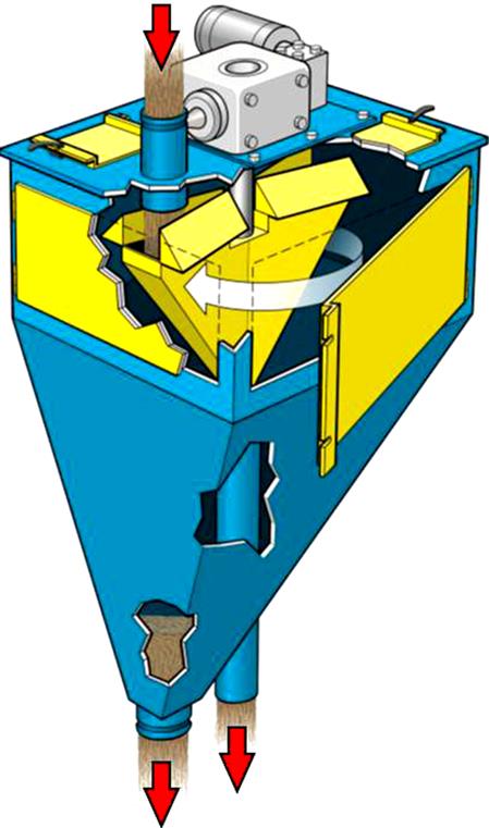
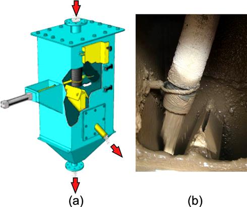
An example of a gravity sampler for slurry flow in horizontal lines, often used for concentrates feeding OSA systems, is shown in Figure 3.9. The internal cutters (single or multiple) are typically located downstream from a flume arrangement that promotes turbulent, well-mixed conditions prior to sampling. The argument is made, however, that any obstacle such as a cutter that changes the flow streamlines will always create some degree of non-probabilistic conditions and introduce bias. Another design often used for control purposes is the pressure pipe sampler shown in Figure 3.10. In an attempt to reduce bias, flow turbulence and increased mixing are introduced using cross-pipe rods prior to sample extraction. The sample may be extracted either straight through in a vertical pressure pipe sampler (Figure 3.10a) or from the Y-section in a horizontal pressure pipe sampler (Figure 3.10b). The coarser the size distribution the greater the chance for increased bias with both gravity and pressure pipe sampler designs.


Poppet samplers (not shown) use a pneumatically inserted sampling pipe to extract the sample from the center of the flow. This is a sampler design that deviates significantly from probabilistic sampling and should therefore be used for liquids and not slurry, if at all.
A cross-belt sampler (Figure 3.11) is designed to mimic stationary reference sampling of a conveyor belt, a probabilistic and very useful technique for bias testing and plant surveys. This belt sampling, however, is difficult to achieve with an automated sampler swinging across a moving conveyor, particularly if the material has fractions of very coarse or very fine material. Small particles may remain on the belt underneath the cutter sides, while coarse lumps may be pushed aside preferentially. These samplers find use on leach pad feed, mill feeds and final product streams (François-Bongarçon and Gy, 2002a; Lyman, et al., 2010). For assay purposes it is possible to analyze the material directly on the belt, thus avoiding some of the physical aspects of sampling to feed an OSA system (e.g., Geoscan-M, Elemental analyzer, Scantech) (see Section 3.3).

Sampling systems for pulp and solids will typically require primary, secondary and possibly tertiary sampling stages. Figure 3.12 and Figure 3.13 show examples of such sampling systems. Once installed, testing should be conducted to validate that the system is bias-free.


Manual or automatic (e.g., using small pumps) in-pulp sampling is a non-probabilistic process and should not be used for metallurgical accounting purposes, but is sometimes necessary for plant surveys and pulp density sampling. An example of a manual in-pulp device is shown in Figure 3.14 and is available in various lengths to accommodate vessel size. One option for reducing random error associated with grab sampling using these samplers is to increase the number of “cuts”, however this does not eliminate the inherent bias of non-probabilistic samplers. An example of a stop-belt manual reference sampler is shown in Figure 3.15. These provide probabilistic samples when used carefully and are very useful for bias testing of automatic samplers and for plant surveys.


Traditional methods for manually extracting a sample increment, such as grab sampling, use of a riffle box, and coning, are inherently non-probabilistic and should be avoided. The caveat being that they may be acceptable if the method is used to treat the entire lot of material, dividing it into two equal sub-lots each time, and repeating the process the required number of times to obtain the final mass needed for analysis. Riffling is inherently biased if the two outside slots lead to the same sub-sample side, or the device feeding the riffle is not exactly the same width as the combined width of all slots or the feeding is slow and uneven. Care must be taken with these methods to avoid segregation leading to bias. The recommended method for dividing samples is to use a rotary table riffle or splitter, as shown in Figure 3.16. The close proximity and radial design of the containers, and constant speed of the table and feeder, ensure that equi-probable splitting is achieved.

3.3 On-line Analysis
On-line analysis enables a change of quality to be detected and corrected rapidly and continuously, obviating the delays involved in off-line laboratory testing. This method also frees skilled staff for more productive work than testing of routine samples. The field has been comprehensively reviewed elsewhere (Kawatra and Cooper, 1986; Braden et al., 2002; Shean and Cilliers, 2011).
3.3.1 On-line Element Analysis
Basically, on-line element analysis consists of a source of radiation that is absorbed by the sample and causes it to give off fluorescent response radiation characteristic of each element. This enters a detector that generates a quantitative output signal as a result of measuring the characteristic radiation of one element from the sample. Through calibration, the detector output signal is used to obtain an assay value that can be used for process control (Figure 3.17).

On-stream Analysis
The benefits of continuous analysis of process streams in mineral processing plants led to the development in the early 1960s of devices for X-ray fluorescence (XRF) analysis of flowing slurry streams. The technique exploits the emission of characteristic “secondary” (or fluorescent) X-rays generated when an element is excited by high energy X-rays or gamma rays. From a calibration the intensity of the emission gives element content.
Two methods of on-line X-ray fluorescence analysis are centralized X-ray (on-stream) and in-stream probe systems. Centralized on-stream analysis employs a single high-energy excitation source for analysis of several slurry samples delivered to a central location where the equipment is installed. In-stream analysis employs sensors installed in, or near, the slurry stream, and sample excitation is carried out with convenient low-energy sources, usually radioactive isotopes (Bergeron and Lee, 1983; Toop et al., 1984). This overcomes the problem of obtaining and transporting representative samples of slurry to the analyzer. The excitation sources are packaged with a detector in a compact device called a probe.
One of the major problems in on-stream X-ray analysis is ensuring that the samples presented to the radiation are representative of the bulk, and that the response radiation is obtained from a representative fraction of this sample. The exciting radiation interacts with the slurry by first passing through a thin plastic film window and then penetrating the sample which is in contact with this window. Response radiation takes the opposite path back to the detector. Most of the radiation is absorbed in a few millimeters depth of the sample, so that the layer of slurry in immediate contact with the window has the greatest influence on the assays produced. Accuracy and reliability depend on this very thin layer being representative of the bulk material. Segregation in the slurry can take place at the window due to flow patterns resulting from the presence of the window surface. This can be eliminated by the use of high turbulence flow cells in the centralized X-ray analyzer.
Centralized analysis is usually installed in large plants, requiring continuous monitoring of many different pulp streams, whereas smaller plants with fewer streams may incorporate probes on the basis of lower capital investment.
Perhaps the most widely known centralized analyzer is the one developed by Outotec, the Courier 300 system (Leskinen et al., 1973). In this system a continuous sample flow is taken from each process slurry to be analyzed. The Courier 300 has now been superseded by the Courier SL series. For example, the Courier 6 SL (Figure 3.13) can handle up to 24 sample streams, with typical installations handling 12–18 streams. The primary sampler directs a part of the process stream to the multiplexer for secondary sampling. The unit combines high-performance wavelength and energy dispersive X-ray fluorescence methods and has an automatic reference measurement for instrument stability and self-diagnostics. The built-in calibration sampler is used by the operator to take a representative and repeatable sample from the measured slurry for comparative laboratory assays.
The measurement sequence is fully programmable. Critical streams can be measured more frequently and more measurement time can be used for the low grade tailings streams. The switching time between samples is used for internal reference measurements, which are used for monitoring and automatic drift compensation.
The probe in-stream system uses an isotope as excitation source. These probes can be single element or multi-element (up to 8, plus % solids). Accuracy is improved by using a well-stirred tank of slurry (analysis zone). Combined with solid state cryogenic (liquid N2) detectors, these probes are competitive in accuracy with traditional X-ray generator systems and can be multiplexed to analyze more than one sample stream. Such devices were pioneered by AMDEL and are now marketed by Thermo Gamma-Metrics. Figure 3.18 shows the TGM in-stream “AnStat” system – a dedicated analyzer with sampling system (Boyd, 2005).

X-ray fluorescence analysis is not effective on light elements. The Outotec Courier 8 SL uses laser-induced breakdown spectroscopy (LIBS) to measure both light and heavy elements. Since light elements are often associated with gangue this analyzer permits impurity content to be tracked.
On-belt Analysis
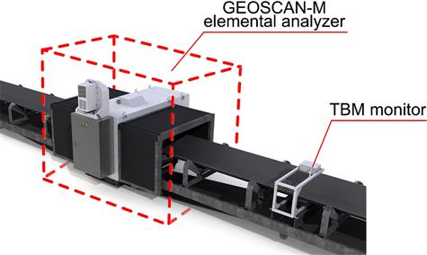
Using a technique known as prompt gamma neutron activation analysis (PGNAA), the GEOSCAN-M (M for minerals applications) is an on-belt, non-contact elemental analysis system for monitoring bulk materials (Figure 3.19) (units specifically designed for the cement and coal industries are also available). By early 2015, over 50 units were operating in minerals applications in iron ore, manganese, copper, zinc-lead and phosphate (Arena and McTiernan, 2011; Matthews and du Toit, 2011; Patel, 2014). A Cf-252 source placed under the belt generates neutrons that pass through the material and interact with the element nuclei to release gamma ray emissions characteristic of the elements. Detectors above the belt produce spectral data, that is, intensity versus energy level. Input from a belt scale provides tonnage weighted averaging of results over time and measurement reporting increments are typically every 2 to 5 minutes. A moisture (TBM) monitor is incorporated to correct for moisture content and allow for elemental analysis on a dry solids basis. Moisture is measured using the microwave transmission technique. A generator below the belt creates a microwave field and free moisture is measured by the phase shift and attenuation.
Laser induced breakdown spectroscopy (LIBS) is also used for on-belt analysis, supplied by Laser Distance Spectrometry (LDS, www.laser-distance-spectrometry.com). In this instrument a laser is directed to the material on the belt and characteristic emissions are detected and converted to element analysis. An advantage is that the analysis includes light elements (Li, Be, etc.). The MAYA M-2010 has been installed in a variety of mining applications.
3.3.2 On-stream Mineral Phase Analysis
Rather than elemental analysis, there is a case to measure actual mineral content as it is the minerals that are being separated. The analysis of phase can be broadly divided into two types: 1. elemental analysis coupled with mineralogical knowledge and mass balancing; and 2. direct determination using diffraction or spectroscopy. The first is essentially adapting the techniques described in Section 3.3.1; the electron beam techniques such as QEMSCAN and MLA (Chapters 1 and 17) use this approach and on-line capability may be possible.
Of the second category X-ray diffraction (XRD) is the common approach and on-line applications are being explored (Anon., 2011). XRD requires that the minerals be crystalline and not too small (>100 nm), and quantitative XRD is problematic due to matrix effects. Spectroscopic techniques include Raman, near infra-red (NIR), nuclear magnetic resonance, and Mössbauer. Their advantage is that the phases do not have to be crystalline. Both NIR and Raman are available as on-line instruments (BlueCube systems). Mössbauer spectroscopy (MS) is particularly useful as a number of mineral phases contain Fe and Fe MS data can be obtained at room temperature. Combining XRD and MS can result in simplifying phase identification (Saensunon et al., 2008). Making such units on-line will be a challenge, however.
The various technologies being developed to identify phases in feeds to ore sorters are another source of on-line measurements. For example, Lessard et al. (2014) describe a dual-energy X-ray transmission method. X-ray transmission depends on the atomic density of the element such that denser elements adsorb more (transmit less). Thus phases containing high density elements can be differentiated from phases containing low density elements by the magnitude of the transmitted intensity. By using two (dual) X-ray energies it is possible to compensate for differences in the volume that is being detected.
3.3.3 On-stream Ash Analysis
The operating principle is based on the concept that when a material is subjected to irradiation by X-rays, a portion of this radiation is absorbed, with the remainder being reflected. The radiation absorbed by elements of low atomic number (carbon and hydrogen) is lower than that absorbed by elements of high atomic number (silicon, aluminum, iron), which form the ash in coal, so the variation of absorption coefficient with atomic number can be directly applied to the ash determination.
A number of analyzers have been designed, and a typical one is shown in Figure 3.20. A representative sample of coal is collected and crushed, and fed as a continuous stream into the presentation unit of the monitor, where it is compressed into a compact uniform bed of coal, with a smooth surface and uniform density. The surface is irradiated with X-rays from a Pu-238 isotope and the radiation is absorbed or back-scattered in proportion to the elemental composition of the sample, the back-scattered radiation being measured by a proportional counter. At the low-energy level of the Pu-238 isotope (15–17 keV), the iron is excited to produce fluorescent X-rays that can be filtered, counted, and compensated. The proportional counter simultaneously detects the back-scattered and fluorescent X-rays after they have passed through an aluminum filter. This filter absorbs the fluorescent X-rays preferentially, its thickness preselected to suit the iron content and its variation. The proportional counter converts the radiation to electrical pulses that are then amplified and counted in the electronic unit. The count-rate of these pulses is converted to a voltage which is displayed and is also available for process control.

A key sensor required for the development of an effective method of controlling coal flotation is one which can measure the ash content of coal slurries. Production units have been manufactured and installed in coal preparation plants (Kawatra, 1985), and due to the development of on-line ash monitors, coupled with an improved knowledge of process behavior, control strategies for coal flotation have been developed (Herbst and Bascur, 1985; Salama et al., 1985; Clarkson, 1986).
3.3.4 On-line Particle Size Analysis
Measuring the size of coarse ore particles on conveyor belts or fine particles in slurries can now be done on-line with appropriate instrumentation. This is covered in Chapter 4.
3.3.5 Weighing the Ore
Many schemes are used for determination of the tonnage of ore delivered to or passing through different sections of a mill. The general trend is toward weighing materials on the move. The predominant advantage of continuous weighing over batch weighing is its ability to handle large tonnages without interrupting the material flow. The accuracy and reliability of continuous-weighing equipment have improved greatly over the years. However, static weighing equipment is still used for many applications because of its greater accuracy.
Belt scales, or weightometers, are the most common type of continuous-weighing devices and consist of one or more conveyor idlers mounted on a weighbridge. The belt load is transmitted from the weighbridge either directly or via a lever system to a load-sensing device, which can be either electrically, mechanically, hydraulically, or pneumatically activated. The signal from the load-sensing device is usually combined with another signal representing belt speed. The combined output from the load and belt-speed sensors provides the flowrate of the material passing over the scale. A totalizer can integrate the flowrate signal with time, and the total tonnage carried over the belt scale can be registered on a digital read-out. Accuracy is normally 1-2% of the full-scale capacity.
It is the dry solids flowrate that is required. Moisture can be measured automatically (see Section 3.3.1). To check, samples for moisture determination are frequently taken from the end of a conveyor belt after material has passed over the weighing device. The samples are immediately weighed wet, dried at a suitable temperature until all hygroscopic (free) water is driven off, and then weighed again. The difference in weight represents moisture and is expressed as:
(3.10)
The drying temperature should not be so high that breakdown of the minerals, either physically or chemically, occurs. Sulfide minerals are particularly prone to lose sulfur dioxide if overheated; samples should not be dried at temperatures above 105°C.
Periodic testing of the weightometer can be made either by passing known weights over it or by causing a length of heavy roller chain to trail from an anchorage over the suspended section while the empty belt is running.
Many concentrators use one master weight only, and in the case of a weightometer this will probably be located at some convenient point between the crushing and the grinding sections. The conveyor feeding the fine-ore bins is often selected, as this normally contains the total ore feed of the plant.
Weighing the concentrates is usually carried out after dewatering, before the material leaves the plant. Weighbridges can be used for material in wagons, trucks, or ore cars. They may require the services of an operator, who balances the load on the scale beam and notes the weight on a suitable form. After tipping the load, the tare (empty) weight of the truck must be determined. This method gives results within 0.5% error, assuming that the operator has balanced the load carefully and noted the result accurately. With recording scales, the operator merely balances the load, then turns a screw which automatically records the weight. Modern scales weigh a train of ore automatically as it passes over the platform, which removes the chance of human error except for occasional standardization. Sampling must be carried out at the same time for moisture determination. Assay samples should be taken, whenever possible, from the moving stream of material, as described earlier, before loading the material into the truck.
Tailings weights are rarely, if ever, measured. They are calculated from the difference in feed and concentrate weights. Accurate sampling of tailings is essential. Mass balance techniques are now routinely used to estimate flows (see Section 3.6).
3.3.6 Mass Flowrate
By combining slurry flowrate and % solids (mass-flow integration), a continuous recording of dry tonnage of material from pulp streams is obtained. The mass-flow unit consists of a flowmeter and a density gauge often fitted to a vertical section of a pipeline carrying the upward-flowing stream. The principal flowmeters are the magnetic-, ultrasonic-, and array-based.
Magnetic Flowmeter
The operating principle of the magnetic flowmeter (Figure 3.21) is based on Faraday’s law of electromagnetic induction, which states that the voltage induced in any conductor as it moves across a magnetic field is proportional to the velocity of the conductor. Thus, providing the pulp completely fills the pipeline, its velocity will be directly proportional to the flowrate. Generally, most aqueous solutions are adequately conductive for the unit and, as the liquid flows through the metering tube and cuts through the magnetic field, an electromotive force (emf) is induced in the liquid and is detected by two small measuring electrodes fitted virtually flush with the bore of the tube. The flowrate is then recorded on a chart or continuously on an integrator. The coil windings are excited by a single-phase AC mains supply and are arranged around the tube to provide a uniform magnetic field across the bore. The unit has the advantage that there is no obstruction to flow, pulps and aggressive liquids can be handled, and it is immune to variations in density, viscosity, pH, pressure, or temperature. A further development is the DC magnetic flowmeter, which uses a pulsed or square excitation for better stability and reduced zero error.

Ultrasonic Flowmeters
Two types of ultrasonic flowmeters are in common use. The first relies on reflection of an ultrasonic signal by discontinuities (particles or bubbles) into a transmitter/receiver ultrasonic transducer. The reflected signal exhibits a change in frequency due to the Doppler Effect that is proportional to the flow velocity; these instruments are commonly called “Doppler flow meters”. As the transducer can be attached to the outside of a suitable pipe section, these meters can be portable.
The second type of meter uses timed pulses across a diagonal path. These meters depend only on geometry and timing accuracy. Hence they can offer high precision with minimal calibration.
Array-based Flowmeters
These operate by using an array of sensors and passive sonar processing algorithms to detect, track, and measure the mean velocities of coherent disturbances traveling in the axial direction of a pipe (Figure 3.22). A coherent disturbance is one that retains its characteristics for an appreciable distance, which in this case is the length of the array of sensors or longer. These coherent disturbances are grouped into three major categories: disturbances conveyed by the flow, acoustic waves in the fluid, and vibrations transmitted via the pipe walls. Each disturbance class travels at a given velocity. For example, the flow will convey disturbances such as turbulent eddies (gases, liquids and most slurries), density variations (pastes), or other fluid characteristics at the rate of the fluid flow. Liquid-based flows rarely exceed 9 m s−1. Acoustic waves in the fluid will typically have a minimum velocity of 75 m s−1 and a maximum velocity of 1500 m s−1. The third group, pipe vibrations, travels at velocities that are several times greater than the acoustic waves. Thus each disturbance class may be clearly segregated based on its velocity.

The velocities are determined as follows: as each group of disturbances pass under a sensor in the array, a signal unique to that group of disturbances is detected by the sensor. In turbulent flow, this signal is generated by the turbulent eddies which exert a miniscule stress on the interior of the pipe wall as they pass under the sensor location. The stress strains the pipe wall and thus the sensor element which is tightly coupled to the pipe wall. Each sensor element converts this strain into a unique electrical signal that is characteristic of the size and energy of the coherent disturbance. By tracking the unique signal of each group of coherent disturbances through the array of sensors, the time for their passage through the array can be determined. The array length is fixed, therefore the passage time is inversely proportional to the velocity. Taking this velocity and the known inner diameter of the pipe, the flow meter calculates and outputs the volumetric flowrate.
This technology accurately measures multiphase fluids (any combination of liquid, solids and gas bubbles), on almost any pipe material including multilayer pipes, in the presence of scale buildup, with conductive or non-conductive fluids, and with magnetic or non-magnetic solids. In addition, the velocity of the acoustic waves, which is also measured, can be used to determine the gas void fraction of bubbles in the pipe. The gas void fraction is the total volume occupied by gas bubbles, typically air bubbles, divided by the interior volume of the pipe. When gas bubbles are present, this measurement is necessary to provide a true non-aerated volumetric flowrate and to compensate for the effect of entrained gas bubbles on density measurements from Coriolis meters or nuclear density meters. This principle can be used to determine void fraction, or gas holdup, in flotation systems (Chapter 12).
Slurry Density
The density of the slurry is measured automatically and continuously in the nucleonic density gauge (Figure 3.23) by using a radioactive source. The gamma rays produced by this source pass through the pipe walls and the slurry at an intensity that is inversely proportional to the pulp density. The rays are detected by a high-efficiency ionization chamber and the electrical signal output is recorded directly as pulp density. Fully digital gauges using scintillation detectors are now in common use. The instrument must be calibrated initially “on-stream” using conventional laboratory methods of density analysis from samples withdrawn from the line.

The mass-flow unit integrates the rate of flow provided by the flowmeter and the pulp density to yield a continuous record of tonnage of dry solids passing through the pipe, given that the specific gravity of the solids comprising the ore stream is known. The method offers a reliable means of weighing the ore stream and removes chance of operator error and errors due to moisture sampling. Another advantage is that accurate sampling points, such as poppet valves (Section 3.2.4), can be incorporated at the same location as the mass-flow unit. Mass-flow integrators are less practicable, however, with concentrate pulps, especially after flotation, as the pulp contains many air bubbles, which lead to erroneous values of flowrate and density. Inducing cyclonic flow of slurry can be used to remove bubbles in some cases.
3.4 Slurry Streams: Some Typical Calculations
Volumetric Flowrate
From the grinding stage onward, most mineral processing operations are carried out on slurry streams, the water and solids mixture being transported through the circuit via pumps and pipelines. As far as the mineral processor is concerned, the water is acting as a transport medium, such that the weight of slurry flowing through the plant is of little consequence. What is of importance is the volume of slurry flowing, as this will affect residence times in unit processes. For the purposes of metallurgical accounting, the weight of dry solids contained within the slurry is important.
If the volumetric flowrate is not excessive, it can be measured by diverting the stream of pulp into a suitable container for a measured period of time. The ratio of volume collected to time gives the flowrate of pulp. This method is ideal for most laboratory and pilot scale operations, but is impractical for large-scale operations, where it is usually necessary to measure the flowrate by online instrumentation.
Volumetric flowrate is important in calculating retention times in processes. For instance, if 120 m3 h−1 of slurry is fed to a flotation conditioning tank of volume 20 m3, then, on average, the retention time of particles in the tank will be (Eq. (3.8)):
Retention time calculations sometimes have to take other factors into account. For example, to calculate the retention time in a flotation cell the volume occupied by the air (the gas holdup) needs to be deducted from the tank volume (see Chapter 12); and in the case of retention time in a ball mill the volume occupied by the slurry in the mill is required (the slurry holdup).
Slurry Density and % Solids
Slurry, or pulp, density is most easily measured in terms of weight of pulp per unit volume. Typical units are kg m−3 and t m−3, the latter having the same numerical value as specific gravity, which is sometimes useful to remember. As before, on flowstreams of significant size, this is usually measured continuously by on-line instrumentation.
Small flowstreams can be diverted into a container of known volume, which is then weighed to give slurry density directly. This is probably the most common method for routine assessment of plant performance, and is facilitated by using a density can of known volume which, when filled, is weighed on a specially graduated balance giving direct reading of pulp density.
The composition of a slurry is often quoted as the % solids by weight (100–% moisture), and can be determined by sampling the slurry, weighing, drying and reweighing, and comparing wet and dry weights (Eq. (3.10)). This is time-consuming, however, and most routine methods for computation of % solids require knowledge of the density of the solids in the slurry. There are a number of methods used to measure this, each method having pros and cons. For most purposes the use of a standard density bottle has been found to be a cheap and, if used with care, accurate method. A 25- or 50-ml bottle can be used, and the following procedure adopted:
1. Wash the density bottle with acetone to remove traces of grease.
3. After cooling, weigh the bottle and stopper on a precision analytical balance, and record the weight, M 1.
4. Thoroughly dry the sample to remove all moisture.
5. Add about 5–10 g of sample to the bottle and reweigh. Record the weight, M 2.
6. Add double distilled water to the bottle until half-full. If appreciable “slimes” (minus 45 μm particles) are present in the sample, there may be a problem in wetting the mineral surfaces. This may also occur with certain hydrophobic mineral species, and can lead to false low density readings. The effect may be reduced by adding one drop of wetting agent, which is insufficient to significantly affect the density of water. For solids with extreme wettability problems, an organic liquid such as toluene can be substituted for water.
7. Place the density bottle in a desiccator to remove air entrained within the sample. This stage is essential to prevent a low reading. Evacuate the vessel for at least 2 min.
8. Remove the density bottle from the desiccator, and top up with double distilled water (do not insert stopper at this stage).
9. When close to the balance, insert the stopper and allow it to fall into the neck of the bottle under its own weight. Check that water has been displaced through the stopper, and wipe off excess water from the bottle. Record the weight, M 3.
10. Wash the sample out of the bottle.
11. Refill the bottle with double distilled water, and repeat procedure 9. Record the weight, M 4.
12. Record the temperature of the water used, as temperature correction is essential for accurate results.
The density of the solids (s, kg m−3) is given by:
(3.11)
where Df=density of fluid used (kg m−3).
Knowing the densities of the pulp and dry solids, the % solids by weight can be calculated. Since pulp density is mass of slurry divided by volume of slurry, then for unit mass of slurry of x % solids by weight, the volume of solids is x/100s and volume of water is (100–x)/100 W then (the 100’s compensating for x in percent):
(3.12a)
or:
(3.12b)
where D=pulp density (kg m−3), and W=density of water (kg m−3).
Assigning water a density of 1000 kg m−3, which is sufficiently accurate for most purposes, gives:
(3.13)
Having measured the slurry volumetric flowrate (F, m3 h−1), the pulp density (D, kg m3), and the density of solids (s, kg m−3), the mass flowrate of slurry can be calculated (FD, kg h−1), and, of more importance, the mass flowrate of dry solids in the slurry (M, kg h−1):
(3.14)
or combining Eqs. (3.13) and (3.14):
(3.15)
The computations are illustrated by examples (Examples 3.4 and 3.5).
Example 3.4
A slurry stream containing quartz is diverted into a 1-liter density can. The time taken to fill the can is measured as 7 s. The pulp density is measured by means of a calibrated balance, and is found to be 1400 kg m−3. Calculate the % solids by weight, and the mass flowrate of quartz within the slurry.
Solution
The density of quartz is 2650 kg m−3. Therefore, from Eq. (3.13), % solids by weight:

The volumetric flowrate:
Therefore, mass flowrate:

Example 3.5
A pump is fed by two slurry streams. Stream 1 has a flowrate of 5.0 m3 h−1 and contains 40% solids by weight. Stream 2 has a flowrate of 3.4 m3 h−1 and contains 55% solids by weight. Calculate the tonnage of dry solids pumped per hour (density of solids is 3000 kg m−3.)
Solution
Slurry stream 1 has a flowrate of 5.0 m3 h−1 and contains 40% solids. Therefore, from a re-arranged form of Eq. (3.13):
thus:
Therefore, from Eq. (3.15), the mass flowrate of solids in slurry stream 1:

Slurry stream 2 has a flowrate of 3.4 m3 h−1 and contains 55% solids. Using the same equations as above, the pulp density of the stream=1579 kg m−3. Therefore, from Eq. (3.14), the mass flowrate of solids in slurry stream 2=1.82 t h−1. The tonnage of dry solids pumped is thus:
In some cases it is necessary to know the % solids by volume, a parameter, for example, sometimes used in mathematical models of unit processes:
(3.16)
Also of use in milling calculations is the ratio of the weight of water to the weight of solids in the slurry, or the dilution ratio. This is defined as:
(3.17)
This is particularly important as the product of dilution ratio and weight of solids in the pulp is equal to the weight of water in the pulp (see also Section 3.7) (Examples 3.6 and 3.7).
Example 3.6
A flotation plant treats 500 t of solids per hour. The feed pulp, containing 40% solids by weight, is conditioned for 5 min with reagents before being pumped to flotation. Calculate the volume of conditioning tank required. (Density of solids is 2700 kg m−3.)
Solution
The volumetric flowrate of solids in the slurry stream:
The mass flowrate of water in the slurry stream

Therefore, the volumetric flowrate of water is 750 m3 h−1.
The volumetric flowrate of slurry=750+185.2
Therefore, for a nominal retention time of 5 min, the volume of conditioning tank should be:
Example 3.7
Calculate the % solids content of the slurry pumped from the sump in Example 3.5.
Solution
The mass flowrate of solids in slurry stream 1 is: 2.73 t h−1
The slurry contains 40% solids, hence the mass flowrate of water:
Similarly, the mass flowrate of water in slurry stream 2:
Total slurry weight pumped:
Therefore, % solids by weight:
3.5 Automatic Control in Mineral Processing
Control engineering in mineral processing continues to grow as a result of more demanding conditions such as low grade ores, economic changes (including reduced tolerance to risk), and ever more stringent environmental regulations, among others. These have motivated technological developments on several fronts such as:
a. Advances in robust sensor technology. On-line sensors such as flowmeters, density gauges, and particle size analyzers have been successfully used in grinding circuit control. Machine vision, a non-invasive technology, has been successfully implemented for monitoring and control of mineral processing plants (Duchesne, 2010; Aldrich et al., 2010; Janse Van Vuuren et al., 2011; Kistner et al., 2013). Some commercial vision systems are VisioRock/Froth (Metso Minerals), FrothMaster (Outotec) and JKFrothCam (JK-Tech Pty Ltd).
Other important sensors are pH meters, level and pressure transducers, all of which provide a signal related to the measurement of the particular process variable. This allows the final control elements, such as servo valves, variable speed motors, and pumps, to manipulate the process variables based on signals from the controllers. These sensors and final control elements are used in many industries besides the minerals industry, and are described elsewhere (Edwards et al., 2002; Seborg et al., 2010).
b. Advances in microprocessor and computer technology. These have led to the development of more powerful Distributed Control Systems (DCS) equipped with user friendly software applications that have facilitated process supervision and implementation of advanced control strategies. In addition, DCS capabilities combined with the development of intelligent sensors have allowed integration of automation tasks such as sensor configuration and fault detection.
c. More thorough knowledge of process behavior. This has led to more reliable mathematical models of various important process units that can be used to evaluate control strategies under different simulated conditions (Mular, 1989; Napier-Munn and Lynch, 1992; Burgos and Concha, 2005; Yianatos et al., 2012).
d. Increasing use of large units, notably large grinding mills and flotation cells. This has reduced the amount of instrumentation and the number of control loops to be implemented. At the same time, however, this has increased the demands on process control as poor performance of any of these large pieces of equipment will have a significant detrimental impact on overall process performance.
Financial models have been developed for the calculation of costs and benefits of the installation of automatic control systems (Bauer et al., 2007; Bauer and Craig, 2008). Benefits reported include energy savings, increased metallurgical efficiency and throughput, and decreased consumption of reagents, as well as increased process stability (Chang and Bruno, 1983; Flintoff et al., 1991; Thwaites, 2007).
The concepts, terminology and practice of process control in mineral processing have been comprehensively reviewed by Ulsoy and Sastry (1981), Edwards et al. (2002) and Hodouin (2011). Some general principles are introduced here, with specific control applications being reviewed in some later chapters.
3.5.1 Hierarchical Multilayer Control System
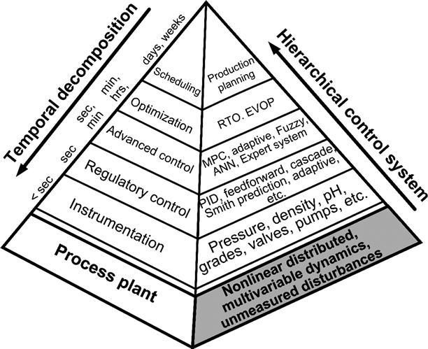
The overall objective of a process control system is to maximize economic profit while respecting a set of constraints such as safe operation, environmental regulations, equipment limitations, and product specifications. The complexity of mineral processing plants, which exhibit multiple interacting nonlinear processes affected by unmeasured disturbances, makes the problem of optimizing the whole plant operation cumbersome, if not intractable. In order to tackle this problem a hierarchical control system, as depicted in Figure 3.24, has been proposed. The objective of this control system structure is to decompose the global problem into simpler, structured subtasks handled by dedicated control layers following the divide-and-conquer strategy. Each control layer performs specific tasks at a different timescale, which provides a functional and temporal decomposition (Brdys and Tatjewski, 2005).
3.5.2 Instrumentation Layer
At the lowest level of the hierarchical control system is the instrumentation layer which is in charge of providing information to the upper control layers about the process status through the use of devices such as sensors and transmitters. At the same time, this layer provides direct access to the process through final control elements (actuators) such as control valves and pumps. Intelligent instrumentation equipped with networking capabilities has allowed the implementation of networks of instruments facilitating installation, commissioning and troubleshooting while reducing wiring costs (Caro, 2009). Examples of industrial automation or fieldbus networks are Profibus-PA, Foundation Fieldbus™, Ethernet/IP and Modbus Plus.
3.5.3 Regulatory Control Layer
The regulatory control layer is implemented in control hardware such as a DCS, PLC (programmable logic controllers) or stand-alone single station field devices. In this control layer, multiple single-input single-output (SISO) control loops are implemented to maintain local variables such as speed, flow or level at their target values in spite of the effect of fast acting disturbances such as pressure and flow variations. In order to achieve a desired regulation performance, the controller executes an algorithm at a high rate. As an example of regulatory control, consider Figure 3.25, which illustrates a froth depth (level) control system for a flotation column. The objective is to regulate the froth depth at its set-point by manipulating the valve opening on the tailing stream to counter the effect of disturbances such as feed and air rate variations. To that end, a level transmitter (LT) senses the froth depth (process variable, PV) based on changes in some physical variables, for example, pressure variations by using a differential pressure sensor, and transmits an electrical signal (e.g., 4–20 mA) proportional to froth depth. The local level controller (LC) compares the desired froth depth (set-point, SP) to the actual measured PV and generates an electric signal (control output, CO) that drives the valve. This mechanism is known as feedback or closed-loop control.

The most widely used regulatory control algorithm is the Proportional plus Integral plus Derivative (PID) controller. It can be found as a standard function block in DCS and PLC systems and also in its stand-alone single station version. There are several types of algorithms available. The standard (also known as non-interacting) algorithm has the following form:
(3.18)
 (3.18)
where CO=controller output; Kc=controller gain; e(t)=deviation of process variable from set-point (tracking error); Ti=integral time constant; Td=derivative time constant; t=time. The process of selecting the parameters of a PID controller, namely Kc, Ti and Td for the standard form, is known as tuning. Although the search for the appropriate PID parameters can be done by trial-and-error, this approach is only acceptable for simple processes having fast dynamics. To design an effective controller, a process model, performance measure, and signal characterization (type of disturbances and set-point) must be considered (Morari and Zafiriou, 1989). Several tuning rules have been proposed since the work of Ziegler and Nichols (1942). A simple set of tuning rules that provides good performance for a wide variety of processes is given by Skogestad (2003). Among PID type controllers PI (Proportional-Integral) is by far the most frequently encountered in industrial applications, mainly because it provides reasonably good performance with only two parameters (Kc, Ti). Application of single parameter, Proportional-only controller, results in steady-state error (offset) which largely limits its application.
Besides tuning, there are other issues the control engineer must deal with when implementing a PID controller. For example, if for some reason the closed-loop is broken, then the controller will no longer act upon the process and the tracking error can be different from zero. The integral part of the controller, then, will increase without having any effect on the process variable. Consequently, when the closed-loop is restored the control output will be too large and it will take a while for the controller to recover. This issue is known as integral windup.
There are situations when a closed-loop system becomes open-loop: (1) the controller is switched to manual mode, and (2) the final control element, such as a valve, saturates (i.e., becomes fully open or fully closed). Figure 3.26 shows a schematic representation of a standard form PID controller equipped with an anti-windup scheme that forces the integral part to track the actual control action when in open loop. The parameter Tt is called the tracking constant and determines the speed at which the integral part will follow the actual control output. To deal effectively with actuator saturation, a model of the actuator is required.

A simple model of a valve, for instance, is that it is fully open when control action is larger than 100% (e.g., >20 mA) and fully closed when less than 0% (e.g., <4 mA), and varies linearly when the control action varies in between.
There are some cases where PID controllers are not sufficient to produce the target performance. In those cases, advanced regulatory control (ARC) techniques may enhance performance. Some ARC strategies used in mineral processing systems include: cascade control, feedforward control, Smith predictor control, and adaptive control. To illustrate the application of these ARC strategies consider a grinding circuit as in Figure 3.27.

Cascade control is built up by nesting control loops. Figure 3.27 shows a cascade control for the regulation of the overflow slurry density, here used as a surrogate of particle size. The density controller (DC) in this case is the primary, also known as the master controller. It calculates a control action based on the deviation of the actual slurry density measurement from its set-point. However, rather than directly acting upon the final control element (valve), it provides a set-point to the inner water flowrate controller FC (secondary or slave controller). This technique has proven useful in attenuating the effect of disturbances occurring in the inner loop (e.g., water pressure variations) on the primary variable (density), especially when the outer process exhibits a transport delay. Moreover, when the inner loop is faster than the outer control loop then the tuning procedure can be carried sequentially starting by tuning the inner controller first (with outer control loop off) and subsequently tuning the primary controller neglecting the inner loop dynamics. Inner feedback control also reduces the effect of actuator nonlinearities, such as valve sticking, and dead band and nonlinear flow characteristics, on the primary control performance. Note that the whole hierarchical control system of Figure 3.27 is actually a cascade control system.
A disadvantage of feedback control is that it compensates for disturbances once they have already affected the process variable, that is, once an error has been produced. Feedforward control takes anticipatory corrective actions to compensate for a major disturbance at the expense of having an extra sensor to measure it. The control engineer has to assess whether the investment in extra instrumentation will be repaid with better regulation.
A typical application of a type of feedforward control is ratio control. Figure 3.27 shows a feedforward ratio control that aims to maintain the solid content (holdup) in the rod mill. Depending on the solid mass flowrate entering the mill measured by a weightometer (WT), a feedforward ratio controller acts by changing the set-point for the water flowrate control loop accordingly.
Processes that exhibit large transport delays relative to their dynamics can seriously limit the achievable performance of any feedback control, regardless of the complexity of the controller. In those cases, PID control performance can be improved by augmenting with a predictor, that is, a mathematical model of the process without the transport delay. This strategy is known as “Smith predictor controller” and it has been successfully applied to improve control performance of solid mass flowrate for SAG mills when manipulating the feed to a conveyor belt (Sbarbaro et al., 2005). In this case the transport delay is a function of the length and speed of the conveyor belt.
Changes in raw material characteristics and/or changes in the operating conditions mean any mathematical model used for controller synthesis may no longer reflect the actual process dynamic behavior. In those cases a control system that modifies controller parameters based on the mismatch between process model and actual process behavior is known as adaptive control (Hodouin and Najim, 1992). This type of “self-tuning” control adapts not only to load-dependent dynamic changes, but also to time-related and/or random dynamic characteristic changes (Rajamani and Hales, 1987; Thornton, 1991; Duarte et al., 1998). The measurements coming from the actual process are compared to the measurements predicted by the model, and the difference is used as the basis for the correction to the model. This correction alters the parameters and states (i.e., a set of variables that determines the state of the process) in the model so as to make the predictions better match those of the actual process. The basis of parameter and state estimation is the recursive least squares algorithm (Ljung, 1999), where the estimator updates its estimates continuously with time as each input arrives, rather than collecting all the information together and processing in a single batch (Figure 3.28).

3.5.4 Advanced Process Control Layer
The control strategy for the grinding section shown in Figure 3.27 where multiple independent local SISO control loops were implemented is known as decentralized control. When the process exhibits severe interaction this decentralized strategy strongly limits the achievable performance and more advanced control strategies are required. A control system that takes interactions explicitly into account is known as centralized multivariable control and it is commonly implemented at the advanced process control layer. This control layer is in charge of keeping secondary variables related to process performance at their optimum, determined by the upper optimization layer, while dealing with interactions and constraints in a dynamic fashion. Receding horizon model based predictive control (MPC) provides a methodology to deal with this type of problem in a systematic way. The main cost associated with MPC is the identification and maintenance of good mathematical models. However, user friendly MPC packages implemented in DCS systems have greatly facilitated these tasks and thus the application of MPC technology in industrial processes. Examples of MPC software packages commercially available are Connoiseur (Invensys), Delta V Predict MPC (Emerson), cpmPlus Expert Optimizer (ABB), BrainWave (Andritz), Profit® Controller (Honeywell) and StarCS MPC (Mintek).
MPC translates a control problem into a dynamic optimization problem over a finite future horizon. A discrete mathematical model is used to generate predictions of the future evolution of the process variable based on current information, future control actions, and assumptions about the future behavior of disturbances. The solution to this optimization problem is a sequence of control moves. Due to the uncertainty in the process model and the disturbances, only the first calculated optimal control move is implemented and the optimization problem is solved again based on new arriving information. This way, the optimization horizon is receding and thus a feedback mechanism is incorporated.
To illustrate MPC, consider a SISO discrete model of the process represented by a difference equation where y, u, and d are the process variable, control output and an unmeasured disturbance, respectively, and a and b are the model parameters:
(3.19)
This model can be used recursively to obtain predictions of the process variable y over a finite time horizon H.
(3.20)
 (3.20)
An optimization problem can then be formulated: find the sequence of future control moves u(t), u(t+1), … , u(t+H–1) that minimizes the deviations of the process output from its reference trajectory while satisfying multiple constraints such as limits on actuator range/rate of change, output constraints, etc. Note that minimization of the control moves is commonly incorporated in the objective function to be minimized, that is:
(3.21)
 (3.21)
where r is the reference trajectory over the time horizon H, and λ an adjustable parameter that weights control moves with respect to tracking errors.
Note that the solution to the optimization problem will be a function of the future values of the disturbance, which are not known in advance. There are different strategies to deal with this issue, a simple way being to assume that the disturbance is constant over the time horizon and takes the same value as its current value d(t), which can be estimated from the difference between the actual measured process variable ymeas(t) and that provided by the model:
(3.22)
where ![]() stands for disturbance estimation. Figure 3.29 illustrates the MPC strategy. Some examples of MPC applications in mineral processing systems include grinding control (Ramasamy et al., 2005; Jonas, 2008; Steyn and Sandrock, 2013), and flotation control (Cortes et al., 2008).
stands for disturbance estimation. Figure 3.29 illustrates the MPC strategy. Some examples of MPC applications in mineral processing systems include grinding control (Ramasamy et al., 2005; Jonas, 2008; Steyn and Sandrock, 2013), and flotation control (Cortes et al., 2008).

Expert Systems
In cases where the identification and maintenance of good mathematical models for the application of MPC technology become unwieldy, expert systems, which do not require an algorithmic mathematical model, are an alternative (Ruel, 2014). Expert systems derive from research into artificial intelligence (AI) and are computer programs that emulate the reasoning of human expertise in a narrowly focused domain (Laguitton and Leung, 1989; Bearman and Milne, 1992). Essentially, they are computer systems that achieve high levels of performance in tasks for which humans would require years of special education, training, or experience. Human operators often make “rule-of-thumb” educated guesses that have come to be known as heuristics. As the expert knowledge is commonly expressed with some degree of uncertainty, ambiguity or even contradiction fuzzy-logic forms an integral part of expert systems.
Fuzzy-logic theory involves the development of an ordered set of fuzzy conditional statements, which provide an approximate description of a control strategy, such that modification and refinement of the controller can be performed without the need for special technical skills. These statements are of the form: if X is A then Y is B, where X and Y are process variables and A and B represent linguistic expressions such “low” and “high”. All the conditional rules taken together constitute a fuzzy decisional algorithm for controlling the plant.
Figure 3.30 illustrates a fuzzy inference-based expert system. It consists of three stages: fuzzyfication, rule based fuzzy inference, and defuzzification. In the fuzzification stage, the operational span of each variable, that is, the range or the universe of discourse as known in AI, is covered by fuzzy sets represented by membership functions labeled with English-like linguistic expressions. Membership functions are usually of triangular, trapezoidal or Gaussian shape. Then, any measurement can be evaluated to determine its degree of membership to each fuzzy set. As a result, a fuzzy sentence like: thickener underflow density is 70% “a little high”, 30% “medium high” and 0% “very low” can be obtained. Then, a set of rules of the form IF-THEN is generated in a process called knowledge acquisition phase. An example of a fuzzy rule for thickener control is: if underflow density is “a little high” then flocculant addition change is “small decrease”. Finally, the last stage of this fuzzy-inference system (defuzzification) converts a fuzzy action such as small decrease of flocculant addition into a crisp value (e.g., 10% decrease).

Harris and Meech (1987) have presented an excellent introduction to Fuzzy Control, showing how it has been applied to a simulation model of a secondary crushing plant. The simplicity of the method allows for its application to systems such as grinding circuits (Hales and Ynchausti, 1997), flotation plants (Osorio et al., 1999), and thickening (Shoenbrunn and Toronto, 1999).
Control systems based on rules with fuzzy logic support have steadily become more ambitious. Van der Spuy et al. (2003) propose an “on-line expert” which will provide both operator training and assistance. Expert systems have also proven useful for selecting which advanced control method might be appropriate, based on a set of rules related to the current operating conditions (Flintoff, 2002).
3.5.5 Optimization Layer
The objective of this control layer is to determine the plant operating point that maximizes economic profit while satisfying a set of constraints. This can be formulated as an optimization problem where an objective function, a scalar positive real-valued function, provides a measure of performance. An example of a potential objective function is the Net Smelter Return (NSR) introduced in Chapter 1. Based on the temporal decomposition of the hierarchical control system depicted in Figure 3.24, this layer assumes the process operates in steady-state and therefore utilizes a stationary nonlinear model of the process to determine the optimum operating conditions.
Figure 3.31 shows a block diagram of a real-time optimization (RTO) layer. A steady-state detection algorithm continuously monitors the process variables for steady-state condition. When this condition is confirmed, the measured data, subject to errors from different sources, are adjusted to satisfy fundamental principles such as those of conservation of mass and/or energy. This process is known as data reconciliation (Hodouin, 2011) (see Section 3.6). The reconciled data are then used to update the process model parameters including unmeasured external inputs in order for the model to represent the actual process condition as accurately as possible.

To deal with complexity, plant optimization is usually broken down into multiple staged local optimizations coordinated by a supervisory system. For example, optimization of the grinding-flotation section can be decomposed into two optimization problems with specific objective functions and interfacing constraints (McIvor and Finch, 1991). A good example of RTO was reported by Holdsworth et al. (2002) for the Greens Creek silver–lead–zinc mine in Alaska. The highly instrumented concentrator carried out frequent on-line mass balances based on the last 2 h of operation. The balanced data were used to calibrate a simple flotation model. The operator could then assess strategies for “moving” metal between low-value bulk concentrate and high-value lead or zinc concentrates with the aid of a simple on-line NSR model. Another application of the RTO-based linear programming technique was proposed to maximize throughput while maintaining product fineness at its target value for a rod-ball grinding section (Lestage et al., 2002). Other optimizing control systems in mineral processing can be found in (Herbst and Bascur, 1984; McKee and Thornton, 1986; Hodouin, 2011).
If an accurate model of the process is not available, a model-free optimization strategy based on evolutionary operation EVOP (Box and Draper, 1998) can be considered. EVOP optimization is based on control action to either continue or reverse the direction of movement of process efficiency by manipulating the set-point of the controller to achieve some higher level of performance. The controlled variables are altered according to a predetermined strategy, and the effect on the process efficiency is computed on-line. If the efficiency is increased as a result of the change, then the next change is made in the same direction, otherwise the direction is reversed; eventually the efficiency should converge to the optimum (Krstev and Golomeov, 1998). Hulthén and Evertsson (2011) implemented an automatic EVOP algorithm that varied eccentric speed on a cone crusher. Although the algorithm pointed in the optimal direction it was found to be too slow to cope with short-term variations such as changes in the feed.
There are cases where primary variables related to economic performance are not available or cannot be measured frequently enough for optimizing control purposes. This can arise for multiple reasons: for example, high cost instrumentation, long sampling measurement delays (e.g., on-stream analyzer, lab analysis), or because the primary variable is a calculated variable (e.g., recovery). In those cases the missing variable can be inferred from a mathematical model using secondary (surrogate) variables that are correlated to the primary variable and measured on-line in real time. These models are known as soft or virtual sensors and their use in a control system is called inferential control.
Models relating secondary to primary variables can be classified into three categories, depending whether the model structure and parameters have a physical meaning. While phenomenological models are derived from first principles, black box models, as their name suggests, provide no insight into the phenomena governing the process. Gray models combine both phenomenological models with empirical relationships. Artificial Neural Networks (ANN), a general class of parametric nonlinear mapping between inputs and outputs, belong to the black box type of model and have been successfully used for developing soft-sensors, due to their ability to learn complex input-output patterns. Some applications of soft-sensor based ANN in mineral processing are particle size estimation of hydrocylone overflow (Sbarbaro et al., 2008), particle size distribution from a conveyor belt using image processing (Ko and Shang, 2011), SAG mill power predictions (Hales and Ynchausti, 1992), and concentrate grade estimation in flotation (González et al., 2003). Soft-sensors based on gray-box modeling through the use of Kalman filter and its extended version have been reported to infer SAG mill parameters (Herbst and Pate, 1996; Apelt et al., 2002) and frother concentration in flotation systems (Maldonado et al., 2010). Statistical methods such as latent variable methods (Principal Component Analysis (PCA), Partial Least Squares (PLS)) have also been implemented to estimate process variables from analysis of digital images. Some examples are the estimation of froth grade and froth properties in flotation systems (Duchesne, 2010; Kistner et al., 2013). González (2010) provides an extensive list of soft-sensing applications in mineral processing.
3.5.6 The Control Room
Control computers are housed in dedicated rooms. It is recognized that many of the systems used within the control room need to be addressed ergonomically using a human, or a user-centered design approach: Figure 3.32 shows a design adhering to several of the ISO 11064 “Control Room Ergonomic Design” standards.

Remote monitoring and control are used in several industries, including some examples in mining: remote operation of mining equipment, such as haul trucks, for example, is standard at many sites. Arguably the main driver of remote “command centers” is the retention of highly skilled workforce in an urban setting. Integrated operations (iOps, https://www.youtube.com/watch?v=qDrObBfv9q8) seeks to integrate the best talents, local and remote, to meet operational challenges. Flintoff et al. (2014) offer some observations on these developments as they relate to mining.
3.6 Mass Balancing Methods
Mass balancing or accounting for phase masses and component mass fractions by phase is critical to many responsibilities of the metallurgical team of any mineral or metal processing plant: troubleshooting/improving/assessing plant performance, monitoring/controlling plant operation, accounting/reporting metal production, and stock movements.
Today, data acquisition and mass balancing are increasingly computerized and automated. Mass balancing techniques have evolved accordingly from the well-known 2-product formula to advanced computerized statistical algorithms that can handle the many situations and issues a metallurgist may have to address when performing mass balance calculations.
The evolution is particularly significant in mass balancing for metal and production accounting and reporting needs. With tighter and more stringent accounting regulations, guidelines and good practices in metal accounting have been generated and published (AMIRA, 2007; Jansen, 2009; Lachance et al., 2012). Statistical reconciliation of excess (redundant) data is nowadays the norm in mass balancing (Reid et al., 1982) and the 2-product formula does not fit any longer with best practices due to its limitations.
This section of Chapter 3 is an introduction to mass balancing and metal accounting, summarizing years of evolution from the basic well-known 2-product formula to computerized advanced statistical techniques. While the n-product formula was used for many years, its limitations and the progress of the information technology sector have made possible the use of more advanced methods. Three of them are reviewed here:
All three methods apply to mass balancing complex flow diagrams and provide a unique set of estimates in the presence of an excess of data.
3.6.1 The n-product Formula
The n-product formula applies to a process unit (or group of process units) with 1 feed and n products, or n feeds and 1 product, or a total of n+1 feed and product streams.
For sake of simplicity, let us start with the 2-product formula before introducing the n-product case. The 2-product formula applies to a process unit or group of process units with one feed and 2 products (a concentrate and a tailings stream, for example (Figure 3.33)), or with 2 feed streams and one product (as in a junction box or mixing unit).

If WF, WC and WT are, respectively, the mass flowrates of feed, concentrate and tailings, then, assuming steady state, the (solids) mass conservation equation is:
(3.23)
Assuming xF, xC, and xT are the assay values of a metal of interest, then a second (or component) mass conservation equation is:
(3.24)
Now assuming WF, xF, xC, and xT are measured, it follows from the previous 2 equations that:
(3.25)
and hence, the mass flowrates of concentrate and tailings are both estimable and the 6 values, WF, WC, WT, xF, xC, and xT, all balance together. Equation (3.25) is known as the 2-product formula.
From the above results, several performance indicators are typically calculated.
The solid split (or its inverse, the ratio of concentration), which states how much of the feed solid reports to the concentrate stream:
(3.26)
The metal recovery, R, which gives how much of the metal contained in the feed has been recovered in the concentrate stream (Chapter 1) and is a measure of the plant metallurgical performance:
(3.27)
The simplicity of the method and resulting equations and the limited amount of data required for providing information on the process performance and efficiency account for the success of the 2-product formula over the years (Example 3.8).
Example 3.8
The feed to a Zn flotation plant assays 3.93% Zn. The concentrate produced assays 52.07% Zn and the tailings 0.49% Zn. Calculate the solid split, ratio of concentration, enrichment ratio, and Zn recovery.
Solution
The solid split (Eq. (3.26)) is:
The ratio of concentration is the inverse of the solid split:
The enrichment ratio (xC/xF) is:
The Zn recovery (Eq. (3.27)) is:

Components other than metal assays can be used, including particle size and percent solids data (see Section 3.7).
By extension of the 2-product formula, the n-product formula works for a process unit or group of process units with one feed and n product streams (or any combination of n+1 streams around the process unit). Assuming the mass flowrate of the feed stream is known, the n-product formula provides a way of calculating the mass flowrates of the n product streams, provided metal assays are known on each of the n+1 streams. The mass conservation equations are:
(3.28)
and
(3.29)
To be solvable the number of required assayed metals depends on n, the number of product streams. There are n unknown mass flowrates and hence n mass conservation equations are needed. Since there is always one equation available that expresses the mass conservation of solids (Eq. (3.28)), then n–1 additional equations are needed (equations of the form of Eq. (3.29)) and therefore n–1 metals need be assayed on the n+1 streams. Table 3.1 summarizes the n-product formula requirements in terms of assayed metals.
Table 3.1
Requirements for n-product Formula
| Number of Product Streams | Number of Required Assayed Metals | Number of Samples |
| 2 | 1 | 3 |
| 3 | 2 | 4 |
| 4 | 3 | 5 |
| n | n–1 | n+1 |
While the 2-product formula remains simple, the formula complexity increases very quickly with n, which explains why its use has been limited to n=4. Mathematically speaking, there exists a matrix formulation to the problem that can easily be computerized.
Sensitivity Analysis
The 2-product formula calculates the values of WC and WT, the concentrate and tailings streams mass flowrates, knowing WF, xF, xC, and xT respectively the feed stream mass flowrate and the metal assay of interest on each of the 3 streams. The measured values of WF, xF, xC, and xT are tainted with measurement errors. The measurement errors are propagated through the calculations on to the values of WC and WT. The following explains how to estimate VC and VT, the variances of WC and WT, knowing VF, Vf, Vc, and Vt, the variances of WF, xF, xC, and xT.
Assuming covariance terms can be neglected, the variance of a function is obtained from its first derivatives:
(3.30)
Applying Eq. (3.30) to the 2-product formula (Eq. (3.25)) gives (all assays and variances as fractions):
(3.31)
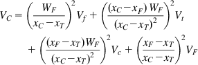 (3.31)
(3.32)
 (3.32)
In the above equations, the difference xC–xT is present in the denominator of each term of the equations. It follows that the calculated variance increases when the xC–xT difference value decreases and hence when the assayed metal is not well separated in the process unit.
Applying Eq. (3.30) to the recovery formula (Eq. (3.27)) gives (again, reminding, all assays and variances as fractions):
(3.33)
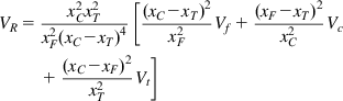 (3.33)
This equation clearly shows that the calculated recovery variance is also strongly dependent on the process unit separation efficiency for the metal of interest (Example 3.9).
Example 3.9
The streams in the Zn flotation plant (Example 3.8) are also assayed for their content in Cu and Fe. The laboratory reports the measured values in Table ex 3.9.
Table ex 3.9
Zinc Flotation Plant Metal Assays (%)
| Feed | Concentrate | Tailings | |
| Zn | 3.93 | 52.07 | 0.49 |
| Cu | 0.16 | 0.66 | 0.14 |
| Fe | 11.57 | 14.67 | 13.09 |

Calculate the recoveries of zinc and copper and provide the expression of their variances as functions of the variances of Zn and Cu assays on all 3 streams.
Solution
The recoveries of Zn and Cu are calculated using Eq. (3.27):
and their variances are provided by Eq. (3.33):
From this numerical example, it is evident that: a) the stream samples that contribute most to the recovery variance are those with the lower assay values (feed and tailings); b) the variance of the least separated metal (Cu) is much higher than the variance of the most separated metal (Zn); and c) when using the 2-product formula, the accuracy of the recovery value comes from the feed and tailings stream assay accuracies rather than from the concentrate. There is a challenge here since these are not necessarily the easiest samples to collect. Worked examples estimating the standard deviation on recovery are given in Example 3.19.
Error Propagation
The n-product formula enables the computation of non-measured mass flowrates from metal assays and from the feed stream flowrate. The n-product formula does not take into account measurement errors; and measurement errors, when present, are propagated onto the calculated mass flowrates.
Example 3.9 provides a good example of error propagations. Table 3.2 displays the calculated values of the solid split using the Zn assay, the Cu assay, and the Fe assay.
Table 3.2
| Feed | Concentrate | Tailings | |
| Zn | 1.0 | 6.7 | 93.3 |
| Cu | 1.0 | 4.5 | 95.5 |
| Fe | 1.0 | −96.2 | 196.2 |

Should the measured assays be free of measurement errors, the solid split values would be identical since, in theory (and reality), there exists only one solid split value. Obviously, the Fe assay is erroneous on at least one of the 3 streams, but it is impossible to identify which one. If each of the Zn and the Cu assays are taken individually, it is not possible to ascertain that the Zn assay or the Cu assay suffers error on one of the 3 samples. It is only because at least 2 metals have been assayed that we can ascertain the presence of measurement errors.
Excess of Data
Example 3.9 data introduces a second limitation of the n-product formula: there is no provision on how to deal with an excess of data. And due to the unavoidable presence of measurement errors, it is not good practice to keep only just sufficient data to apply the n-product formula even when the data set includes the metals best separated in the process unit.
Since an excess of data reveals measurement errors, there is a need for a mass balancing method which can deal with data in excess.
More than One Process Unit
Another limitation of the n-product formula is that it deals with only one process unit or group of process units. The formula does not apply to more complex problems.
In the process flow diagram of Figure 3.34, the feed flowrate is measured and Cu has been assayed on each of the 6 stream samples. The question is: can we apply the n-product formula to estimate the non-measured flowrates and complete the mass balance?

Applying the 2-product formula on process unit A, it is possible to calculate the flowrate of each of the 2 outgoing streams. Considering that the flowrate of the feed stream to process unit B is now known, the 2-product formula provides values of the 2 outgoing stream flowrates of process unit B.
As a result of the above calculations, we now have an excess of data for process unit C, since the only unknown flowrate is for the outgoing stream. Consequently the 2-product formula fails to complete the mass balance calculation.
It is worth noticing that selecting any other path in the applications of the 2-product formula would have ended up in the same situation: an excess of data preventing the completion of the mass balance calculation. There are various ways to address this kind of issue and to complete the mass balance, but the point is that the n-product formula is not sufficient.
No Correction of Measurement Errors
The n-product formula closes the mass balance and provides values for the non-measured flowrates; hence it gives access to key performance indicators such as the solid split and the metal recovery.
We have seen, however, that the n-product formula propagates measurement errors onto the calculated flowrate values. Another drawback is that it does not correct the measurement errors. In the example of Table 3.2 and without any indication about the uncertainties associated with Zn and Cu assays, there is no reason to trust more the solid split value calculated with the Zn assays than with the Cu assays. Obviously there is something very wrong with the Fe assays, but there is no way to identify which of the feed, concentrate or tailings stream sample is culprit.
For all the above reasons, the n-product formula cannot be considered any longer as a mass balancing method. The following section presents a more sound approach to mass balancing in presence of measurement errors.
3.6.2 Node Imbalance Minimization
In the Node Imbalance Minimization method, the mass conservation equations are written considering the deviation to rigorous mass conservation due to measurement errors (Finch and Matwijenko, 1977; Lynch, 1977; Tipman et al., 1978; Klimpel, 1979). For the simple case of a process unit with one feed and two products, the mass conservation equations are:
(3.34)
(3.35)
where the W’s stand for the mass flowrates and the x’s for the metal assays; IW and Ix are the node imbalances (errors) for the mass of solids and the mass of metal of interest, respectively. Additional equations can be written for each assayed metal of interest and/or each process unit.
In a given mass balance, the total number of mass conservation equations is therefore a function of the number of process units and metals assayed. For the flow diagram of Figure 3.34 and assuming three metals have been assayed, the total number of mass conservation equations would be: 3 process units×(1 solid equation+3 assay equations)=12 equations. Assuming that the feed flowrate is known, then the total number of unknown is 5: the solid mass flowrates of the other streams.
Typically there are more equations than unknowns and, as a consequence, there is not a unique solution that satisfies all equations. The best mass flowrate estimates, ![]() , are those which minimize the following criterion:
, are those which minimize the following criterion:
(3.36)