
Classification
Classification, as defined by Heiskanen, is a method of separating mixtures of minerals into two or more products on the basis of the velocity with which the particles fall through a fluid medium. The carrying fluid can be a liquid or a gas. In mineral processing, this fluid is usually water, and wet classification is generally applied to mineral particles that are considered too fine (<200 µm) to be sorted efficiently by screening. As such, this chapter will only discuss wet classification. A description of the historical development of both wet and dry classification is given by Lynch and Rowland.
Keywords
Principles; hydrocyclones; sedimentation classifiers; hydraulic classifiers; classifier performance
9.1 Introduction
Classification, as defined by Heiskanen (1993), is a method of separating mixtures of minerals into two or more products on the basis of the velocity with which the particles fall through a fluid medium. The carrying fluid can be a liquid or a gas. In mineral processing, this fluid is usually water, and wet classification is generally applied to mineral particles that are considered too fine (<200 µm) to be sorted efficiently by screening. As such, this chapter will only discuss wet classification. A description of the historical development of both wet and dry classification is given by Lynch and Rowland (2005).
Classifiers are nearly always used to close the final stage of grinding and so strongly influence the performance of these circuits (Chapter 7). Since the velocity of particles in a fluid medium is dependent not only on the size, but also on the specific gravity and shape of the particles, the principles of classification are also important in mineral separations utilizing gravity concentrators (Chapter 10).
9.2 Principles of Classification
9.2.1 Force Balance
When a solid particle falls freely in a vacuum, there is no resistance to the particle’s motion. Therefore, if it is subjected to a constant acceleration, such as gravity, its velocity increases indefinitely, independent of size and density. Thus, a lump of lead and a feather fall at exactly the same rate in a vacuum.
In a viscous medium, such as air or water, there is resistance to this movement and this resistance increases with velocity. When equilibrium is reached between the gravitational force and the resistant force from the fluid, the body reaches its terminal velocity and thereafter falls at a uniform rate.
The nature of the resistance, or drag force, depends on the velocity of the descent. At low velocities, motion is smooth because the layer of fluid in contact with the body moves with it, while the fluid a short distance away is motionless. Between these two positions is a zone of intense shear in the fluid all around the descending particle. Effectively, all resistance to motion is due to the shear forces, or the viscosity of the fluid, and is hence called viscous resistance. At high velocities the main resistance is due to the displacement of fluid by the body, with the viscous resistance being relatively small; this is known as turbulent resistance. Whether viscous or turbulent resistance dominates, the acceleration of particles in a fluid rapidly decreases and the terminal velocity is reached relatively quickly.
A particle accelerates according to Newton’s well-known equation where ![]() is the net force acting on a particle,
is the net force acting on a particle, ![]() the mass of the particle, and
the mass of the particle, and ![]() the acceleration of the particle:
the acceleration of the particle:
(9.1)
As mass, a combination of a particle’s size and density, is a factor on the particle acceleration, it is common for fine high-density material, such as gold or galena, to be misclassified and report to the same product with the coarser low density particles. This occurrence will be further discussed in Section 9.2.4.
The classification process involves the balancing of the accelerating (gravitational, centrifugal, etc.) and opposing (drag, etc.) forces acting upon particles, so that the resulting net force has a different direction for fine and coarse particles. Classifiers are designed and operated so that the absolute velocities, resulting from the total net force, cause particles to be carried into separable products. Forces acting upon particles can include:
• Gravitational or electrostatic field force
• Inertial force, centrifugal force, and Coriolis force (only in rotational systems)
An example of a classifier is a sorting column, in which a fluid is rising at a uniform rate (Figure 9.1). Particles introduced into the sorting column either sink or rise according to whether their terminal velocities, a result of the net force, are greater or smaller than the upward velocity of the fluid. The sorting column therefore separates the feed into two products—an overflow consisting of particles with terminal velocities smaller than the velocity of the fluid and an underflow or spigot product containing particles with terminal velocities greater than the rising velocity.

9.2.2 Free Settling
Free settling refers to the sinking of particles in a volume of fluid which is large with respect to the total volume of particles, hence particle–particle contact is negligible. For well-dispersed pulps, free settling dominates when the percentage by weight of solids is less than about 15% (Taggart, 1945).
Consider a spherical particle of diameter d and density ρs falling under gravity in a viscous fluid of density ρf under free-settling conditions, that is, ideally in a fluid of infinite size. The particle is acted upon by three forces: a gravitational force acting downward (taken as positive direction), an upward buoyant force due to the displaced fluid, and a drag force D acting upward (see Figure 9.1). Following Newton’s law of motion in Eq. (9.1), the equation of motion of the particle is therefore:
(9.2)
 (9.2)
(9.2)
where m is the mass of the particle, m′ the mass of the displaced fluid, x the particle velocity, and g the acceleration due to gravity. When terminal velocity is reached, acceleration (dx/dt) is equal to zero, and hence:
(9.3)
Therefore, using the volume and density of a sphere:
(9.4)
Stokes (1891) assumed that the drag force on a spherical particle was entirely due to viscous resistance and deduced the expression:
(9.5)
where η is the fluid viscosity and v the terminal velocity.
Hence, substituting in Eq. (9.4) we derive:
or solving for the terminal velocity
(9.6)
This expression is known as Stokes’ law.
Newton assumed that the drag force was entirely due to turbulent resistance, and deduced:
(9.7)
Substituting in Eq. (9.4) gives:
(9.8)
This is Newton’s law for turbulent resistance.
The range for which Stokes’ law and Newton’s law are valid is determined by the dimensionless Reynolds number (Chapter 4). For Reynolds numbers below 1, Stokes’ law is applicable. This represents, for quartz particles settling in water, particles below about 60 µm in diameter. For higher Reynolds numbers, over 1,000, Newton’s law should be used (particles larger than about 0.5 cm in diameter). There is, therefore, an intermediate range of Reynolds numbers (and particle sizes), which corresponds to the range in which most wet classification is performed, in which neither law fits experimental data. In this range there are a number of empirical equations that can be used to estimate the terminal velocity, some of which can be found in Heiskanen (1993).
Stokes’ law (Eq. (9.6)) for a particular fluid can be simplified to:
(9.9)
and Newton’s law (Eq. (9.8)) can be simplified to:
(9.10)
where k1 and k2 are constants, and (ρs−ρf) is known as the effective density of a particle of density ρs in a fluid of density ρf.
9.2.3 Hindered Settling
As the proportion of solids in the pulp increases above 15%, which is common in almost all mineral classification units, the effect of particle–particle contact becomes more apparent and the falling rate of the particles begins to decrease. The system begins to behave as a heavy liquid whose density is that of the pulp rather than that of the carrier liquid; hindered-settling conditions now prevail. Because of the high density and viscosity of the slurry through which a particle must fall, in a separation by hindered settling the resistance to fall is mainly due to the turbulence created (Swanson, 1989). The interactions between particles themselves, and with the fluid, are complex and cannot be easily modeled. However, a modified form of Newton’s law can be used to determine the approximate falling rate of the particles, in which ρp is the pulp density:
(9.11)
9.2.4 Effect of Density on Separation Efficiency
The aforementioned laws show that the terminal velocity of a particle in a particular fluid is a function of the particle size and density. It can be concluded that:
1. If two particles have the same density, then the particle with the larger diameter has the higher terminal velocity.
2. If two particles have the same diameter, then the heavier (higher density) particle has the higher terminal velocity.
As the feed to most industrial classification devices will contain particles with varying densities, particles will not be classified based on size alone. Consider two mineral particles of densities ρa and ρb and diameters da and db, respectively, falling in a fluid of density ρf at exactly the same settling rate (their terminal velocity). Hence, from Stokes’ law (Eq. (9.9)), for fine particles:
or
(9.12)
This expression is known as the free-settling ratio of the two minerals, that is, the ratio of particle size required for the two minerals to fall at equal rates.
Similarly, from Newton’s law (Eq. (9.8)), the free-settling ratio of large particles is:
(9.13)
The general expression for free-settling ratio can be deduced from Eqs. (9.12) and (9.13) as:
(9.14)
where n=0.5 for small particles obeying Stokes’ law and n=1 for large particles obeying Newton’s law. The value of n lies in the range 0.5–1 for particles in the intermediate size range of 50 µm to 0.5 cm (Example 9.1).
Example 9.1
Consider a binary mixture of galena (specific gravity 7.5) and quartz (s.g. 2.65) particles being classified in water. Determine the free-settling ratio (a) from Stokes’ law and (b) from Newton’s law. What do you conclude?
Solution
a. For small particles, obeying Stokes’ law, the free-settling ratio (Eq. (9.12)) is:
That is, a particle of galena will settle at the same rate as a particle of quartz which has a diameter 1.99 times larger than the galena particle.
b. For particles obeying Newton’s law, the free-settling ratio (Eq. (9.13)) is:
Conclusion: The free-settling ratio is larger for coarse particles obeying Newton’s law than for fine particles obeying Stokes’ law.
The result in Example 9.1 means that the density difference between the particles has a more pronounced effect on classification at coarser size ranges. This is important where gravity concentration is being utilized. Over-grinding of the ore must be avoided, such that particles are fed to the separator in as coarse a state as possible, so that a rapid separation can be made, exploiting the enhanced effect of specific gravity difference. Since the enhanced gravity effect also means that fine heavy minerals are more likely to be recycled and overground in conventional ball mill-classifier circuits, it is preferable where possible to use open circuit rod mills for the primary coarse grind feeding a gravity circuit.
When considering hindered settling, the lower the density of the particle, the greater is the effect of the reduction of the effective density (ρs–ρf). This then leads to a greater reduction in falling velocity. Similarly, the larger the particle, the greater is the reduction in falling rate as the pulp density increases. This is important in classifier design; in effect, hindered-settling reduces the effect of size, while increasing the effect of density on classification. This is illustrated by considering a mixture of quartz and galena particles settling in a pulp of density 1.5. The hindered-settling ratio can be derived from Eq. (9.11) as:
(9.15)
Therefore, in this system:
A particle of galena will thus fall in the pulp at the same rate as a particle of quartz, which has a diameter 5.22 times as large. This compares with the free-settling ratio, calculated as 3.94 for turbulent resistance (Example 9.1).
The hindered-settling ratio is always greater than the free-settling ratio, and the denser the pulp, the greater is the ratio of the diameter of equal settling particles. For quartz and galena, the greatest hindered-settling ratio that we can attain practically is about 7.5. Hindered-settling classifiers are used to increase the effect of density on the separation, whereas free-settling classifiers use relatively dilute suspensions to increase the effect of size on the separation (Figure 9.2). Relatively dense slurries are fed to certain gravity concentrators, particularly those treating heavy alluvial sands. This allows high tonnages to be treated and enhances the effect of specific gravity difference on the separation. The efficiency of separation, however, may be reduced since the viscosity of a slurry increases with density. For separations involving feeds with a high proportion of particles close to the required density of separation, lower slurry densities may be necessary, even though the density difference effect is reduced.

As the pulp density increases, a point is reached where each mineral particle is covered only with a thin film of water. This condition is known as a quicksand, and because of surface tension, the mixture is a perfect suspension and does not tend to separate. The solids are in a condition of full teeter, which means that each grain is free to move, but is unable to do so without colliding with other grains and as a result stays in place. The mass acts as a viscous liquid and can be penetrated by solids with a higher specific gravity than that of the mass, which will then move at a velocity impeded by the viscosity of the mass.
A condition of teeter can be produced in a classifier sorting column by putting a constriction in the column, either by tapering the column or by inserting a grid into the base. Such hindered-settling sorting columns are known as teeter chambers. Due to the constriction, the velocity of the introduced water current is greatest at the bottom of the column. A particle falls until it reaches a point where its falling velocity equals that of the rising current. The particle can now fall no further. Many particles reach this condition, and as a result, a mass of particles becomes trapped above the constriction and pressure builds up in the mass. Particles move upward along the path of least resistance, which is usually the center of the column, until they reach a region of lower pressure at or near the top of the settled mass; here, under conditions in which they previously fell, they fall again. As particles from the bottom rise at the center, those from the sides fall into the resulting void. A general circulation is established, the particles being said to teeter. The constant jostling of teetering particles has a scouring effect which removes any entrained or adhering slimes particles, which then leave the teeter chamber and pass out through the classifier overflow. Clean separations can therefore be made in such classifiers. The teeter column principle is also exploited in some coarse particle flotation cells (Chapter 12).
The analysis in this section has assumed, directly or implicitly, that the particles are spherical. While this is never really true, the resulting broken particle shapes are often close enough to spherical for the general findings above to apply. The obvious exceptions are ores containing flakey or fibrous mineral such as talc, mica, and some serpentines. Shape in those cases will influence the classification behavior.
9.2.5 Effect of Classifier Operation on Grinding Circuit Behavior
Classifiers are widely employed in closed-circuit grinding operations to enhance the size reduction efficiency. A typical ball mill-classifier arrangement is seen in Figure 7.38 (Chapter 7). The benefits of classification can include: improved comminution efficiency; improved product (classifier overflow) quality; and greater control of the circulating load to avoid overloading the circuit (Chapter 7). The improvement in efficiency of the grinding circuit is seen as either a reduction in energy consumption or increase in throughput (capacity). The main increase in efficiency is due to the reduction of overgrinding. By removing the finished product size particles from the circuit they are not subject to unnecessary further grinding (overgrinding), which is a waste of comminution energy. This, combined with the recycling of unfinished (oversize) particles, results in the circuit product (classifier overflow) having a narrower size distribution than is the case for open circuit grinding. This narrow size distribution and restricted amount of excessively fine material benefits downstream mineral separation processes. Other benefits come from reduced particle–particle contact cushioning from fines in the grinding mill and less misplaced coarse material in the overflow, which would reduce downstream efficiencies. Therefore, classifier performance is critical to the optimal running of a mineral processing plant.
9.3 Types of Classifiers
Although they can be categorized by many features, the most important is the force field applied to the unit: either gravitational or centrifugal. Centrifugal classifiers have gained widespread use as classifying equipment for many different types of ore. In comparison, gravitational classifiers, due to their low efficiencies at small particle sizes (<70 µm), have limited use as classifiers and are only found in older plants or in some specialized cases. Table 9.1 outlines the key differences between the two types of classifiers and further highlights the benefits of centrifugal classifiers. Many types of classifiers have been designed and built, and only some common ones will be introduced. A more comprehensive guide to the major types of classification equipment used in mineral processing can be found elsewhere (Anon., 1984; Heiskanen, 1993; Lynch and Rowland, 2005).
Table 9.1
A Comparison of Key Parameters for Centrifugal and Gravitational Classifiers
| Item | Centrifugal Classifiers | Gravitational Classifiers |
| Capacity | High | Low |
| Cut-size | Fine—Coarse | Coarse |
| Capacity/cut-size dependency | Yes | No |
| Energy consumption | High (feed pressure) | Low |
| Initial investment | Low | High |
| Footprint | Small | Large |
9.4 Centrifugal Classifiers—The Hydrocyclone
The hydrocyclone, commonly abbreviated to just cyclone, is a continuously operating classifying device that utilizes centrifugal force to accelerate the settling rate of particles. It is one of the most important devices in the minerals industry, its main use in mineral processing being as a classifier, which has proved extremely efficient at fine separation sizes. Apart from their use in closed-circuit grinding, cyclones have found many other uses, such as de-sliming, de-gritting, and thickening (dewatering). The reasons for this include their simplicity, low investment cost, versatility, and high capacity relative to unit size.
Hydrocyclones are available in a wide range of sizes, depending on the application, varying from 2.5 m in diameter down to 10 mm. This corresponds to cut-sizes of 300 µm down to 1.5 µm, with feed pressures varying from 20 to about 200 kPa (3–30 psi). The respective flowrates vary from 2 m3 s−1 in a large unit to 2.5×10⁻⁵ m3 s−1 in a small unit. Units can be installed on simple supports as single units or in clusters (“cyclopacs”) (Heiskanen, 1993).
9.4.1 Basic Design and Operation
A typical hydrocyclone (Figure 9.3) consists of a conically shaped vessel, open at its apex (also known as spigot or underflow), joined to a cylindrical section, which has a tangential feed inlet. The top of the cylindrical section is closed with a plate through which passes an axially mounted overflow pipe. The pipe is extended into the body of the cyclone by a short, removable section known as the vortex finder. The vortex finder forces the feed to travel downward, which prevents short-circuiting of feed directly into the overflow. The impact of these design parameters on performance is discussed further in Section 9.4.5.
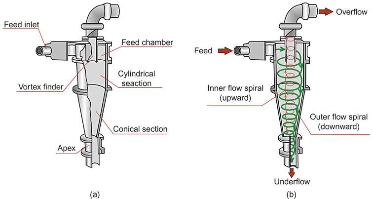
The feed is introduced under pressure through the tangential entry, which imparts a swirling motion to the pulp. This generates a vortex in the cyclone, with a low-pressure zone along the vertical axis. An air core develops along the axis, normally connected to the atmosphere through the apex opening, but in part created by dissolved air coming out of solution in the zone of low pressure.
The conventional understanding is that particles within the hydrocyclone’s flow pattern are subjected to two opposing forces: an outward acting centrifugal force and an inwardly acting drag (Figure 9.4). The centrifugal force developed accelerates the settling rate of the particles, thereby separating particles according to size and specific gravity (and shape). Faster settling particles move to the wall of the cyclone, where the velocity is lowest, and migrate down to the apex opening. Due to the action of the drag force, the slower-settling particles move toward the zone of low pressure along the axis and are carried upward through the vortex finder to the overflow.

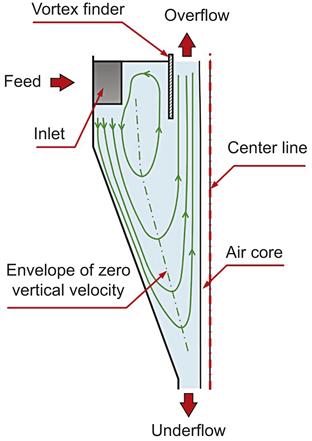
The existence of an outer region of downward flow and an inner region of upward flow implies a position at which there is no vertical velocity. This applies throughout the greater part of the cyclone body, and an envelope of zero vertical velocity should exist throughout the body of the cyclone (Figure 9.5). Particles thrown outside the envelope of zero vertical velocity by the greater centrifugal force exit via the underflow, while particles swept to the center by the greater drag force leave in the overflow. Particles lying on the envelope of zero velocity are acted upon by equal centrifugal and drag forces and have an equal chance of reporting either to the underflow or overflow. This concept should be remembered when considering the cut-point described later.
Experimental work by Renner and Cohen (1978) has shown that classification does not take place throughout the whole body of the cyclone. Using a high-speed probe, samples were taken from several selected positions within a 150-mm diameter cyclone and were subjected to size analysis. The results showed that the interior of the cyclone may be divided into four regions that contain distinctively different size distributions (Figure 9.6).

Essentially unclassified feed exists in a narrow region, A, adjacent to the cylinder wall and roof of the cyclone. Region B occupies a large part of the cone of the cyclone and contains fully classified coarse material, that is, the size distribution is practically uniform and resembles that of the underflow (coarse) product. Similarly, fully classified fine material is contained in region C, a narrow region surrounding the vortex finder and extending below the latter along the cyclone axis. Only in the toroid-shaped region D does classification appear to be taking place. Across this region, size fractions are radially distributed, so that decreasing sizes show maxima at decreasing radial distances from the axis. These results, however, were taken with a cyclone running at low pressure, so the region D may be larger in production units.
9.4.2 Characterization of Cyclone Efficiency
The Partition Curve
The most common method of representing classifier efficiency is by a partition curve (also known as a performance, efficiency, or selectivity curve). The curve relates the weight fraction of each particle size in the feed which reports to the underflow to the particle size. It is the same as the partition curve introduced for screening (Chapter 8). The cut-point, or separation size, is defined as the size for which 50% of the particles in the feed report to the underflow, that is, particles of this size have an equal chance of going either with the overflow or underflow (Svarovsky and Thew, 1992). This point is usually referred to as the d50 size.
It is observed in constructing the partition curve for a cyclone that the partition value does not appear to approach zero as particle size reduces, but rather approaches some constant value. To explain, Kelsall (1953) suggested that solids of all sizes are entrained in the coarse product liquid, bypassing classification in direct proportion to the fraction of feed water reporting to the underflow. For example, if the feed contains 16 t h−1 of material of a certain size, and 12 t h−1 reports to the underflow, then the percentage of this size reporting to the underflow, and plotted on the partition curve, is 75%. However, if, say, 25% of the feed water reports to the underflow, then 25% of the feed material will short-circuit with it; therefore, 4 t h−1 of the size fraction will short-circuit to the underflow, and only 8 t h−1 leave in the underflow due to classification. The corrected recovery of the size fraction is thus:
The uncorrected, or actual, partition curve can therefore be corrected by utilizing Eq. (9.16):
(9.16)
where C is the corrected mass fraction of a particular size reporting to underflow, S the actual mass fraction of a particular size reporting to the underflow, and Rw/u the fraction of the feed liquid that is recovered in the coarse product (underflow) stream, which defines the bypass fraction. The corrected curve thus describes particles recovered to the underflow by true classification and introduces a corrected cut-size, d50c. Kelsall’s assumption has been questioned, and Flintoff et al. (1987) reviewed some of the arguments. However, the Kelsall correction has the advantages of simplicity, utility, and familiarity through long use.
The construction of the actual and corrected partition curves can be illustrated by means of an example. The calculations are easily performed in a spreadsheet (Example 9.2).
Example 9.2
a. Determine the actual partition curve and actual d50 for the cyclone data in Example 3.15.
b. Determine the corrected partition curve and corrected d50c.
As a reminder, the grinding circuit in Example 3.15 is

Solution
a. Using the same symbolism as in Example 3.15 then the partition value S is given by:
From the size distribution data using the generalized least squares minimization procedure, the solids split (recovery) to underflow (U/F) is 0.619. From this, data reconciliation was executed and the adjusted size distribution data are given in Table ex 9.2 along with the actual partition (S) and the corrected partition (C) values.
Table ex 9.2
Adjusted Size Distribution Data and Partition Values
| Size Interval (μm) | Mean Size (μm) | CF | COF | CUF | Partition, S | Corrected, C |
| +592 | 8.27 | 0.23 | 13.21 | 98.9 | 98.3 | |
| −592+419 | 498 | 4.86 | 0.54 | 7.51 | 95.7 | 93.6 |
| −419+296 | 352 | 6.77 | 0.94 | 10.35 | 94.6 | 92.1 |
| −296+209 | 249 | 7.04 | 2.81 | 9.64 | 84.8 | 77.6 |
| −209+148 | 176 | 11.38 | 7.67 | 13.66 | 74.3 | 62.2 |
| −148+105 | 125 | 13.91 | 13.21 | 14.35 | 63.9 | 46.9 |
| −105+74 | 88 | 11.09 | 11.7 | 10.71 | 59.8 | 40.9 |
| −74+53 | 63 | 9.86 | 14.78 | 6.83 | 42.9 | 16.0 |
| −53+37 | 44 | 5.57 | 9.33 | 3.26 | 36.2 | 6.2 |
| −37 | 21.25 | 38.79 | 10.48 | 30.5 | −2.2 | |
| 100 | 100 | 100 |

Specimen calculation of S and mean particle size:
For the −592+419 µm size class:
The mean size is calculated by taking the geometric mean; for example, for the −592+419 size class this is (592×419)0.5=498 µm.
The partition curve is then constructed by plotting the S values (as % in this case) versus the mean particle size, as done in Figure ex 9.2-S.

From the actual partition curve the cut-point d50 is about 90 µm.
b. Example 3.18 showed that the water split (recovery) to underflow was 0.32 (32%). From the actual partition curve in Figure ex 9.2-S this appears to be a reasonable estimate of the bypass fraction. Using this bypass value the corrected partition C values are computed and the corrected partition curve constructed which is included in the figure.
Specimen calculation:
For the −209+148 µm size class:
From the corrected partition curve the d50c is about 120 µm.
Modern literature, including manufacturer’s data, usually quotes the corrected d50 with the subscript “c” dropped. Some care in reading the literature is therefore required. To avoid confusion, the designation d50c will be retained.
Although not demonstrated here, the partition curve is often plotted against d/d50, that is, making the size axis nondimensional—a reduced or normalized size—giving rise to a reduced partition curve.
The exponential form of the curves has led to several fitting models (Napier-Munn et al., 1996). One of the most common (Plitt, 1976) is:
(9.17)
where K is a constant, d the mean particle size, and m the “sharpness” of separation. By introducing C=0.5 at d=d50c and rearranging Eq. (9.17) gives K:
thus:
(9.18a)
and:
(9.18b)
The normalized size is evident in Eq. (9.18a). By fitting data to Eq. (9.18a), the two unknowns, d50c and m, can be estimated. For instance, for Example 9.2 the fitted values (rounded) are: d50c=125 µm and m=1.7.
Sharpness of Cut
The value of m in Eq. (9.18a) is one measure of the sharpness of the separation. The value is determined by the slope of the central section of the partition curve; the closer the slope is to vertical, the higher the value of m and the greater the classification efficiency. Perfect classification would give m=∞; but in reality m values are rarely above 3. The slope of the curve can be also expressed by taking the points at which 75% and 25% of the feed particles report to the underflow. These are the d75 and d25 sizes, respectively. The sharpness of separation, or the so-called imperfection, I, is then given by (where the actual or corrected d50 may be used):
(9.19)
Multidensity Feeds
Inspection of the partition curve in Example 9.2 (Figure ex 9.2-S) shows a deviation at about 100 μm which we chose to ignore by passing a smooth curve through the data, implying, perhaps, some experimental uncertainty. In fact, the deviation is real and is created by classifying feeds with minerals of different specific gravity. In this case the feed is a Pb–Zn ore with galena (s.g. 7.5), sphalerite (4.0), pyrite (5.0), and a calcite/dolomite non-sulfide gangue, NSG (2.85). The individual mineral classification curves can be generated from the metal assay on each size fraction using the following:
(9.20)
where subscript i refers to size class i (which we did not need to specify before) and subscript i,M refers to metal (or mineral) assay M in size class i. The calculations are illustrated using an example (Example 9.3).
Example 9.3
Solution
a. The table and the calculation of the partition values for galena (Si,Pb) calculated using Eq. (9.20) are shown in Table ex 9.3.
Specimen calculation:
For the −53+37 μm size class:
The actual partition curves for all minerals are given in Figure ex 9.3-S.
b. The total solids circulating load CLTot and total galena circulating load CLTot,Pb are given by, respectively (see Example 3.15):

Table ex 9.3
Size Distribution and Pb Assay by Size for the Same Circuit as in Example 9.2
| Size Interval (μm) | Mean Size | CF | COF | CUF | Si,Pb | |||
| wt% | %Pb | wt% | %Pb | wt% | %Pb | |||
| +592 | 8.27 | 1.33 | 0.23 | 1.41 | 13.21 | 1.32 | 98.1 | |
| −592 + 419 | 498 | 4.86 | 1.02 | 0.54 | 1.3 | 7.51 | 1 | 93.8 |
| −419 + 296 | 352 | 6.77 | 1.73 | 0.94 | −0.16 | 10.35 | 1.84 | 100.7 |
| −296 + 209 | 249 | 7.04 | 2.55 | 2.81 | −0.12 | 9.64 | 3.02 | 100.4 |
| −209 + 148 | 176 | 11.38 | 3.19 | 7.67 | 0.25 | 13.66 | 4.21 | 98.1 |
| −148 + 105 | 125 | 13.91 | 3.83 | 13.21 | 0.22 | 14.35 | 5.87 | 97.9 |
| −105 + 74 | 88 | 11.09 | 8.14 | 11.7 | 0.35 | 10.71 | 13.36 | 98.1 |
| −74 + 53 | 63 | 9.86 | 9.21 | 14.78 | 1.02 | 6.83 | 20.07 | 93.4 |
| −53 + 37 | 44 | 5.57 | 6.77 | 9.33 | 2.29 | 3.26 | 14.64 | 78.3 |
| −37 | 21.25 | 3.55 | 38.79 | 3.09 | 10.48 | 4.59 | 39.5 | |
| Head | 100 | 4.29 | 100 | 1.66 | 100 | 5.91 | 85.3 | |

(Note, the “head” row gives the total Pb assay for the stream; and that data reconciliation was not constrained to zero on the Pb assay giving a couple of small negative values in the COF column and consequently Si,Pb values slightly larger than 100%.)

The circulating load of galena is thus 3.56 (5.78/1.63) times that of the solids.
From Example 9.3 it is evident that the high-density galena preferentially reports to the underflow. The minerals, in fact, classify according to their density. Treating the elemental assay curves to be analogous with their associated minerals has the implication that they are liberated, free minerals. This is not entirely true, after all, the purpose of the grinding circuit is to liberate, so in the cyclone feed liberation is unlikely to be complete. It is better to refer to mineral-by-size curves, which does not imply liberated minerals. The analysis can be extended to determine the corrected partition curves and the corresponding m and d50c,M values, which we can then use as a first approximation for the associated minerals. In doing so we find the following values: m=2.2 for all minerals, and d50c,M equals 37 μm for galena, 66 μm for pyrite; 89 μm for sphalerite, and 201 μm for NSG. The m value shows the sharpness of separation is higher for the minerals than for the total solids (m=1.7, Example 9.2). By inspection, the d50c,M values correspond well with the hindered settling expression, from Eq. (9.15). For example, the ratio d50c,NSG: d50c,Ga is 5.4, which is close to the value calculated for the hindered settling of essentially this pair of minerals. It is this density effect, concentrating heavy minerals in the circulating stream, which gives the opportunity for recovery from this stream (or other streams inside the circuit), using gravity separation devices or flash flotation.
Unusual Partition Curves
“Unusual” refers to deviations from the simple exponential form, which can range from inflections to the curve displaying a minimum and maximum (Laplante and Finch, 1984; Kawatra and Eisele, 2006). The partition curve in Example 9.2 illustrates the phenomena: the inflection at about 100 μm was initially ignored in favor of a smooth curve, suggesting, perhaps, experimental error. Example 9.3 shows that the inflection in the total solids curve is because it is the sum of the mineral partition curves (weighted for the mineral content); below 100 μm the NSG is no longer being classified and the solids curve shifts over to reflect the continuing classification of the denser minerals. The “unusual” nature of the curve is even more evident in series cyclones where the downstream (secondary) cyclone receives overflow from the primary cyclone, which now comprises fine dense mineral particles and coarse light mineral particles.
The impact of the component minerals is also evident in the m values: that for the mineral curves is higher than for the solids, and the correspondence to the exponential model, Eq. (9.18a), is better for the minerals than for the solids. It should be remembered when determining m that a low value may not indicate performance that needs improving, as the component minerals may be comparatively quite sharply classified.
Apart from density, the shape of the particles in the feed is also a factor in separation. Flakey particles such as mica often reporting to the overflow, even though they may be relatively coarse. Wet classification of asbestos feeds can reveal similar unusual overall partition curves as for density, this time the result of the shape: fibrous asbestos minerals, and the granular rock particles.
Another “unusual” feature of the partition curve sometimes reported that is not connected to a density (or shape) effect is a tendency for the curve to bend up toward the fine end (Del Villar and Finch, 1992). Called a “fish-hook” by virtue of its shape, it is well recognized in mechanical air classifiers (Austin et al., 1984). Connected to the bypass, the notion is that the fraction reporting to the underflow is size-dependent, that the finer the particles the closer they split in the same proportion as the water, thus bending the partition curve upward (the fish-hook) at the finer particle sizes to intercept the Y-axis at Rw/u. Whether the fish-hook is real or not continues to attract a surprising amount of literature (Bourgeois and Majumder, 2013; Nageswararao, 2014).
Cyclone Overflow Size Distribution
Although partition curves are useful in assessing and modeling classifier performance, the minerals engineer is usually more interested in knowing fineness of grind (i.e., cyclone overflow particle size distribution) than the cyclone cut-size. Simple relationships between fineness of grind and the partition curve of a hydrocyclone have been developed by Arterburn (1982) and Kawatra and Seitz (1985).
Figure 9.7(a) shows the evolution of size distribution of the solids from the feed to product streams for the grinding circuit in Example 9.2; and Figure 9.7(b) shows the size distribution of the solids and the minerals in the cyclone overflow for the same circuit. The latter shows the much finer size distribution of the galena (P80,Pb~45 μm) compared to the solids (P80~120 μm) and the NSG (P80,NSG~130 µm) due to the high circulating load, and thus additional grinding, of the galena. It is this observation which gives rise to the argument introduced Chapter 7 that the grinding circuit treating a high-density mineral component can be operated at a coarse solids P80, as the high-density mineral will be automatically ground finer, and the grind instead could be made the P80 of the target mineral for recovery.

This density effect in cyclones (or any classification device) is often taken to be a reason to consider screening which is density independent. This is a good point at which to compare cyclones with screens.
9.4.3 Hydrocyclones Versus Screens
Hydrocyclones have come to dominate classification when dealing with fine particle sizes in closed grinding circuits (<200 µm). However, recent developments in screen technology (Chapter 8) have renewed interest in using screens in grinding circuits. Screens separate on the basis of size and are not directly influenced by the density spread in the feed minerals. This can be an advantage. Screens also do not have a bypass fraction, and as Example 9.2 has shown, bypass can be quite large (over 30% in that case). Figure 9.8 shows an example of the difference in partition curve for cyclones and screens. The data is from the El Brocal concentrator in Peru with evaluations before and after the hydrocyclones were replaced with a Derrick Stack Sizer® (see Chapter 8) in the grinding circuit (Dündar et al., 2014). Consistent with expectation, compared to the cyclone the screen had a sharper separation (slope of curve is higher) and little bypass. An increase in grinding circuit capacity was reported due to higher breakage rates after implementing the screen. This was attributed to the elimination of the bypass, reducing the amount of fine material sent back to the grinding mills which tends to cushion particle–particle impacts.

Changeover is not one way, however: a recent example is a switch from screen to cyclone, to take advantage of the additional size reduction of the denser payminerals (Sasseville, 2015).
9.4.4 Mathematical Models of Hydrocyclone Performance
A variety of hydrocyclone models have been proposed to estimate the key relationships between operating and geometrical variables for use in design and optimization, with some success. These include empirical models calibrated against experimental data, as well as semi-empirical models based on equilibrium orbit theory, residence time, and turbulent flow theory. Progress is also being made in using computational fluid dynamics to model hydrocyclones from first principles (e.g., Brennan et al., 2003; Nowakowski et al., 2004; Narasimha et al., 2005). All the models commonly used in practice are still essentially empirical in nature.
Bradley model
Bradley’s seminal book (1965) listed eight equations for the cut-size, and the number has increased significantly since then. Bradley’s equation based on the equilibrium orbit hypothesis (Figure 9.4) was:
(9.21)
 (9.21)
where Dc is the cyclone diameter, η the fluid viscosity, Qf the feed flowrate, ρs the solids density, ρl the fluid density, n a hydrodynamic constant (0.5 for particle laminar flow), and k a constant incorporating other factors, particularly cyclone geometry, which must be estimated from experimental data. Equation (9.21) describes some of the process trends well, but cannot be used directly in design or operational situations.
Empirical Models
A variety of empirical models were constructed in the previous century to predict the performance of hydrocyclones (e.g., Leith and Licht, 1972). More recently, models have been proposed by, among others, Nageswararao et al. (2004) and Kraipech et al. (2006). The most widely used empirical models are probably those of Plitt (1976) and its later modified form (Flintoff et al., 1987), and Nageswararao (1995). These models, based on a phenomenological description of the process with numerical constants determined from large databases, are described in Napier-Munn et al. (1996) and were reviewed and compared by Nageswararao et al. (2004).
Plitt’s modified model for the corrected cut-size d50c in micrometers is:
(9.22)
 (9.22)
where Dc, Di, Do, and Du are the inside diameters of the cyclone, inlet, vortex finder, and apex, respectively (cm), η the liquid viscosity (cP), Cv the feed solids volume concentration (%), h the distance between apex and end of vortex finder (cm), k a hydrodynamic exponent to be estimated from data (default value for laminar flow 0.5), Qf the feed flowrate (l min−1), and ρs the solids density (g cm−3). Note that for noncircular inlets, ![]() where A is the cross-sectional area of the inlet (cm2).
where A is the cross-sectional area of the inlet (cm2).
The equation for the volumetric flowrate of slurry to the cyclone Qf is:
(9.23)
where P is the pressure drop across the cyclone in kilopascals (1 psi=6.895 kPa). The F1 and F2 in Eqs. (9.22) and (9.23) are material-specific constants that must be determined from tests with the feed material concerned. Plitt also reports equations for the flow split between underflow and overflow, and for the sharpness of separation parameter m in the corrected partition curve.
Nageswararao’s model includes correlations for corrected cut-size, pressure-flowrate, and flow split, though not sharpness of separation. It also requires the estimate of feed-specific constants from data, though first approximations can be obtained from libraries of previous case studies. This requirement for feed-specific calibration emphasizes the important effect that feed conditions have on hydrocyclone performance.
Asomah and Napier-Munn (1997) reported an empirical model that incorporates the angle of inclination of the cyclone, as well as explicitly the slurry viscosity, but this has not yet been validated in the large-scale use which has been enjoyed by the Plitt and Nageswararao models.
A useful general approximation for the flowrate in a hydrocyclone is
(9.24)
Flowrate and pressure drop together define the useful work done in the cyclone:
(9.25)
where Q is the flowrate (m3 h−1); P the pressure drop (kPa); and Dc the cyclone diameter (cm). The power can be used as a first approximation to size the pump motor, making allowances for head losses and pump efficiency.
These models are easy to incorporate in spreadsheets, and so are particularly useful in process design and optimization using dedicated computer simulators such as JKSimMet (Napier-Munn et al., 1996) and MODSIM (King, 2012), or the flowsheet simulator Limn (Hand and Wiseman, 2010). They can also be used as a virtual instrument or “soft sensor” (Morrison and Freeman, 1990; Smith and Swartz, 1999), inferring cyclone product size from geometry and operating variables as an alternative to using an online particle size analyzer (Chapter 4).
Computational Models
With advances in computer hardware and software, considerable progress has been made in the fundamental modeling of hydrocyclones. The multiphase flow within a hydrocyclone consists of solid particles, which are dispersed throughout the fluid, generally water. In addition, an air core is present. Such multiphase flows can be studied using a combination of Computational Fluid Dynamics (CFD) and Discrete Element Method (DEM) techniques (see Chapter 17).
The correct choice of the turbulence, multiphase (air–water interaction), particle drag, and contact models are essential for the successful modeling of the hydrocyclone. The highly turbulent swirling flows, along with the complexity of the air core and the relatively high feed percent solids, incur large computational effort. Choices are therefore made based on a combination of accuracy and computational expense. Studies have included effects of short-circuiting flow, motion of different particle sizes, the surging phenomena, and the “fish-hook” effect as well as particle–particle, particle–fluid, and particle–wall interactions in both dense medium cyclones (Chapter 11) and hydrocyclones.
The data required to validate numerical models can be obtained through methods such as particle image velocimetry and laser Doppler velocimetry. These track the average velocity distributions of particles, as opposed to Lagrangian tracking, where individual particles of a dispersed phase can be tracked in space and time. Wang et al. (2008) used a high-speed camera to record the motion of a particle with density 1,140 kg m−3 in water in a hydrocyclone. The two-dimensional particle paths obtained showed that local or instantaneous instabilities in the flow field can have a major effect on the particle trajectory, and hence on the separation performance of the hydrocyclone. Lagrangian tracking includes the use of positron emission particle tracking (PEPT), which is a more recent development in process engineering. PEPT locates a point-like positron emitter by cross-triangulation (see Chapter 17). Chang et al. (2011) studied the flow of a particle through a hydrocyclone using PEPT with an 18 F radioactive tracer and could track the particle in the cyclone with an accuracy of 0.2 mm ms−1.
9.4.5 Operating and Geometric Factors Affecting Cyclone Performance
The empirical models and scale-up correlations, tempered by experience, are helpful in summarizing the effects of operating and design variables on cyclone performance. The following process trends generally hold true:
Cut-size (inversely related to solids recovery)
• Increases with cyclone diameter
• Increases with feed solids concentration and/or viscosity
• Increases with correct cyclone size selection
• Decreases with feed solids concentration and/or viscosity
Flow split of water to underflow
• Increases with larger apex or smaller vortex finder
• Decreases with inclined cyclones (especially low pressure)
• Increases with cyclone diameter
• Decreases (at a given pressure) with feed solids concentration and/or viscosity
Since the operating variables have an important effect on the cyclone performance, it is necessary to avoid fluctuations, such as in flowrate and pressure drop, during operation. Pump surging should be eliminated either by automatic control of level in the sump, or by a self-regulating sump, and adequate surge capacity should be installed to eliminate flowrate fluctuations.
The feed flowrate and the pressure drop across the cyclone are related (Eq. (9.22)). The pressure drop is required to enable design of the pumping system for a given capacity or to determine the capacity for a given installation. Usually the pressure drop is determined from a feed-pressure gauge located on the inlet line some distance upstream from the cyclone. Within limits, an increase in feed flowrate will improve fine particle classification efficiency by increasing the centrifugal force on the particles. All other variables being constant, this can only be achieved by an increase in pressure and a corresponding increase in power, since this is directly related to the product of pressure drop and capacity. Since increase in feed rate, or pressure drop, increases the centrifugal force, finer particles are carried to the underflow, and d50 is decreased, but the change has to be large to have a significant effect. Figure 9.9 shows the effect of pressure on the capacity and cut-point of cyclones.

The effect of increase in feed pulp density is complex, as the effective pulp viscosity and degree of hindered settling is increased within the cyclone. The sharpness of the separation decreases with increasing pulp density and the cut-point rises due to the greater resistance to the swirling motion within the cyclone, which reduces the effective pressure drop. Separation at finer sizes can only be achieved with feeds of low solids content and large pressure drop. Normally, the feed concentration is no greater than about 30% solids by weight, but for closed-circuit grinding operations, where relatively coarse separations are often required, high feed concentrations of up to 60% solids by weight are often used, combined with low-pressure drops, often less than 10 psi (68.9 kPa). Figure 9.10 shows that feed concentration has an important effect on the cut-size at high pulp densities.

In practice, the cut-point is mainly controlled by the cyclone design variables, such as those of the inlet, vortex-finder, and apex openings, and most cyclones are designed such that these are easily changed.
The area of the inlet determines the entrance velocity and an increase in area increases the flowrate. The geometry of the feed inlet is also important. In most cyclones the shape of the entry is developed from circular cross section to rectangular cross section at the entrance to the cylindrical section of the cyclone. This helps to “spread” the flow along the wall of the chamber. The inlet is normally tangential, but involuted feed entries are also common (Figure 9.11). Involuted entries are said to minimize turbulence and reduce wear. Such design differences are reflected in proprietary cyclone developments such as Weir Warman’s CAVEX® and Krebs’ gMAX® units.

The diameter of the vortex finder is an important variable. At a given pressure drop across the cyclone, an increase in the diameter of the vortex finder will result in a coarser cut-point and an increase in capacity.
The size of the apex opening determines the underflow density and must be large enough to discharge the coarse solids that are being separated by the cyclone. The orifice must also permit the entry of air along the axis of the cyclone to establish the air vortex. Cyclones should be operated at the highest possible underflow density, since unclassified material (the bypass fraction) leaves the underflow in proportion to the fraction of feed water leaving via the underflow. Under correct operating conditions, the discharge should form a hollow cone spray with a 20–30° included angle (Figure 9.12(a)). Air can then enter the cyclone, the classified coarse particles will discharge freely, and solids concentrations greater than 50% by weight can be achieved. Too small apex opening can lead to the condition known as “roping” (Figure 9.12(b)), where an extremely thick pulp stream of the same diameter as the apex is formed, and the air vortex may be lost, the separation efficiency will fall, and oversize material will discharge through the vortex finder. (This condition is sometimes encouraged where a very high underflow solids concentration is required, but is otherwise deleterious: the impact of this “tramp” oversize on downstream flotation operations can be quite dramatic (Bahar et al., 2014)). Too large an apex orifice results in the larger hollow cone pattern seen in Figure 9.12(c). The underflow will be excessively dilute and the additional water will carry unclassified fine solids that would otherwise report to the overflow. The state of operation of a cyclone is important to optimize both grinding efficiency and downstream separation processes, and online sensors are now being incorporated to identify malfunctioning cyclones (Cirulis and Russell, 2011; Westendorf et al., 2015).

Some investigators have concluded that the cyclone diameter has no effect on the cut-point and that for geometrically similar cyclones the efficiency curve is a function only of the feed material characteristics. The inlet and outlet diameters are the critical design variables, the cyclone diameter merely being the size of the housing required to accommodate these apertures (Lynch et al., 1974, 1975; Rao et al., 1976). This is true where the inlet and outlet diameters are essentially proxies for cyclone diameter for geometrically similar cyclones. However, from theoretical considerations, it is the cyclone diameter that controls the radius of orbit and thus the centrifugal force acting on the particles. As there is a strong interdependence between the aperture sizes and cyclone diameter, it is difficult to distinguish the true effect, and Plitt (1976) concluded that the cyclone diameter has an independent effect on separation size.
For geometrically similar cyclones at constant flowrate, d50 ∝ diameterx, but the value of x is open to much debate. The value of x using the Krebs–Mular–Jull model is 1.875, for Plitt’s model it is 1.18, and Bradley (1965) concluded that x varies from 1.36 to 1.52.
9.4.6 Sizing and Scale-Up of Hydrocyclones
In practice, the cut-point is determined to a large extent by the cyclone size (diameter of cylindrical section). The size required for a particular application can be estimated from empirical models (discussed below), but these tend to become unreliable with extremely large cyclones due to the increased turbulence within the unit, and it is therefore more common to choose the required model by referring to manufacturers’ charts, which show capacity and separation size range in terms of cyclone size. A typical performance chart is shown in Figure 9.13 (where the D designation refers to cyclone diameter in inches). This is for Krebs cyclones, operating at less than 30% feed solids by weight, and with solids specific gravity in the range 2.5–3.2.

Since fine separations require small cyclones, which have only small capacity, enough have to be connected in parallel if to meet the capacity required; these are referred to as clusters, batteries, nests, or cyclopacs (Figure 9.14). Cyclones used for de-sliming duties are usually very small in diameter, and a large number may be required if substantial flowrates must be handled. The de-sliming plant at the Mr. Keith Nickel concentrator in Western Australia has 4,000 such cyclones. The practical problems of distributing the feed evenly and minimizing blockages have been largely overcome by the use of Mozley cyclone assemblies. A 16×51 mm (16×2 in.) assembly is shown in Figure 9.15. The feed is introduced into a housing via a central inlet at pressures of up to 50 psi (344.8 kPa). The housing contains 16 2-in. cyclones, which have interchangeable spigot and vortex finder caps for precise control of cut-size and underflow density. The feed is forced through a trash screen and into each cyclone without the need for separate distributing ports (Figure 9.16). The overflow from each cyclone leaves via the inner pressure plate and leaves the housing through the single overflow pipe on the side. The assembly design reduces maintenance, the removal of the top cover allowing easy access so that individual cyclones can be removed (for repair or replacement) without disconnecting feed or overflow pipework.


Since separation at large particle size requires large diameter cyclones with consequent high capacities, in some cases, where coarse separations are required, cyclones cannot be utilized, as the plant throughput is not high enough. This is often a problem in pilot plants where simulation of the full-size plant cannot be achieved, as scaling down the size of cyclones to allow for smaller capacity also reduces the cut-point produced.
Scale-Up of Hydrocyclones
A preliminary scale-up from a known situation (e.g., a laboratory or pilot plant test) to the unknown (e.g., a full production installation) can be done via the basic relationships between cut-size, cyclone diameter, flowrate, and pressure drop. These are:
(9.26)
and
(9.27)
where P is pressure drop, Q the flowrate, Dc the cyclone diameter, the subscripts 1 and 2 indicate the known and scale-up applications respectively, and n1–6 are constants which are a function of the flow conditions. The theoretical values (for dilute slurries and laminar flow in small cyclones) are: n1=1.5, n2=0.5, n3=0.5, n4=0.25, n5=2.0, and n6=4.0. The constants to be used in practice will depend on conditions and which model is favored. In particular, at a given flowrate high feed solids concentrations will substantially influence both cut-size (increase) and pressure drop (decrease). There is no general consensus, but in most applications the following values will give more realistic predictions: n1=1.54, n2=0.43, n3=0.72, n4=0.22, n5=2.0, and n6=3.76.
These relationships tell us that the diameter, flowrate, and pressure must be considered together. For example, cut-size cannot be scaled purely on cyclone diameter, as a new diameter will bring either a new flowrate or pressure or both. For example, if it is desired to scale to a larger cyclone at the same cut-size, then ![]() and
and ![]() .
.
Classification efficiency can sometimes be improved by arranging several cyclones in series to retreat overflow, underflow, or both. Svarovsky and Thew (1984) have pointed out that if N cyclones with identical classification curves are arranged in series, each treating the overflow of the previous one, then the overall recovery of size d to the combined coarse product, Rd(T), is given by:
(9.28)
where Rd=recovery of size d in one cyclone.
Sizing of Hydrocyclones—Arterburn Technique
Arterburn (1982) published a method, based on the performance of a “typical” Krebs cyclone, which allows for the cyclone size (i.e., diameter) to be estimated for a given application. Using a series of empirical and semi-empirical relationships, the method relates the overflow P80 to the cut-point, d50c, of a “base” cyclone, which is related to cyclone size. An example calculation illustrates the procedure (Example 9.4).
Example 9.4
Select (a) the size and (b) number of cyclones for a ball mill circuit for the following conditions:
Solution
a. Size of cyclone (Dc)
Step 1: Estimate the cut-size for the application.
Arterburn gives a relationship between cut-size for the application and the P80:
Step 2: Determine a generic or base cut-size, d50c (base) from the application, d50c (appl):
where the Cs are correction factors. The relationship changes the specific application to a cyclone operating under base conditions, which is therefore independent of the specific application operating parameters. (Olson and Turner (2002) introduce some additional correction factors reflective of cyclone design.)
The first correction term (C1) is for the influence of the concentration of solids in the feed slurry:
where V is the % solids by volume.
The second correction (C2) is for the influence of pressure drop (ΔP, kPa) across the cyclone, measured by taking the difference between the feed pressure and the overflow pressure:
The final correction (C3) is for the effect of solids specific gravity:
where ρs and ρl are the specific gravity of solid and liquid (usually taken as water, ρl=1). (Arterburn uses Stokes’ law for particles of different densities but equal terminal velocities (Eq. (9.12)), with the reference being a quartz particle of specific gravity 2.65 in water.)
Step 3: Estimate size (diameter) of cyclone from d50c (base) using:

The cyclone sizes in Figure 9.13 are in inches; from those shown the closest, but larger, selection is 26 in. (D-26). From the pressure drop-capacity chart (Figure 9.13) a D-26 unit is suited to the target separation as the d50c (appl) range is 70–150 μm.
From Figure 9.13 a D-26 cyclone can treat about 300 m3 h−1. Thus to handle the target volumetric flowrate of 1,000 m3 h−1 we need (1,000/300), that is, four cyclones.
The cyclone size is the main choice for preliminary circuit design purposes. Variables, such as diameter of vortex finder, inlet, and apex, also affect separation (discussed in Section 9.4.5). Accordingly, most cyclones have replaceable vortex finders and apexes with different sizes available, and adjustments by operations will be made to provide the final design.
Sizing of Hydrocyclones—Mular–Jull Model
Mular and Jull (1980) developed empirical formulae from the graphical information for “typical” cyclones, relating d50c to the operating variables for cyclones of varying diameter. A “typical” cyclone has an inlet area of about 7% of the cross-sectional area of the feed chamber, a vortex finder of diameter 35–40% of the cyclone diameter, and an apex diameter normally not less than 25% of the vortex-finder diameter.
The equation for the cyclone cut-point is:
(9.29)
 (9.29)
Equations such as these have been used in computer-controlled grinding circuits to infer cut-points from measured data, but their use in this respect is declining with the increased use of online particle size monitors (Chapter 4). Their value, however, remains in the design and optimization of circuits by the use of computer simulation, which greatly reduces the cost of assessing circuit options.
Sizing of Hydrocyclones—Simulation Packages
A complement to the above methods of sizing cyclones is to use a simulation package such as those mentioned earlier (JKSimMet, MODSIM, or Limn). These packages incorporate empirical cyclone models such as those by Plitt and Nageswararao and can be used for optimizing processing circuits incorporating cyclones (Morrison and Morrell, 1998).
9.5 Gravitational Classifiers
Gravitational classifiers are best suited for coarser classification and are often used as dewatering and washing equipment. They are simple to operate and have low energy requirements, but capital outlay is relatively high compared to cyclones. Gravitational classifiers can be further categorized into two broad groups, depending on the direction of flow of the carrying current: if the fluid movement is horizontal and forms an angle with the particle trajectory, the classification is called sedimentation classification; if the fluid movement and particle settling directions are opposite, the classification is called hydraulic or counter flow. Sedimentation, or horizontal current, classifiers are essentially of the free-settling type and accentuate the sizing function. On the other hand, hydraulic, or vertical current, classifiers are usually hindered-settling types and so increase the effect of density on the separation.
9.5.1 Sedimentation Classifiers
Nonmechanical Sedimentation Classifiers
As the simplest form of classifier, there is little attempt to do more than separate the solids from the liquid, and as such they are sometimes used as dewatering units in small-scale operations. Therefore, they are not suitable for fine classification or if a high separation efficiency is required. They are often used in the aggregate industry to de-slime coarse sand products. The principle of the settling cone is shown in Figure 9.17. The pulp is fed into the tank as a distributed stream, with the spigot discharge valve, S, initially closed. When the tank is full, overflow of water and slimes commences, and a bed of settled sand builds until it reaches the level shown. The spigot valve is now opened and sand is discharged at a rate equal to that of the input. Classification by horizontal current action takes place radially across zone D from the feed pipe to the overflow lip. The main difficulty in operation of such a device is the balancing of the sand discharge and deposition rates; it is virtually impossible to maintain a regular discharge of sand through an open pipe under the influence of gravity. Many different designs of cone have been introduced to overcome this problem (Taggart, 1945).

In the “Floatex” separator, which is essentially a hindered-settling classifier over a dewatering cone, automatic control of the coarse lower discharge is governed by the specific gravity of the teeter column. The use of the machine as a de-sliming unit and in upgrading coal and mica, as well as its possible application in closed-circuit classification of metalliferous ores, is discussed by Littler (1986).
Mechanical Sedimentation Classifiers
This term describes classifiers in which the material of lower settling velocity is carried away in a liquid overflow, and the material of higher settling velocity is deposited on the bottom of the unit and is transported upward against the flow of liquid by some mechanical means. The principle components of a mechanical classifier are shown in Figure 9.18.

Mechanical classifiers have seen use in closed-circuit grinding operations and in the classification of products from ore-washing plants (Chapter 2). In washing plants, they act more or less as sizing devices, as the particles are essentially unliberated and so are of similar density. In closed-circuit grinding, they have a tendency to return small dense particles to the mill, that is, the same as noted for cyclones. They have also been used to densify dense media (Chapter 11).
The pulp feed is introduced into the inclined trough and forms a settling pool in which coarse particles of high falling velocity quickly reach the bottom of the trough. Above this, coarse sand is a quicksand zone where hindered settling takes place. The depth and shape of this zone depends on the classifier action and on the feed pulp density. Above the quicksand is a zone of essentially free-settling material, comprising a stream of pulp flowing horizontally across the top of the quicksand zone from the feed inlet to the overflow weir, where the fines are removed.
The settled sands are conveyed up the inclined trough by a mechanical rake or by a helical screw. The conveying mechanism also serves to keep fine particles in suspension in the pool by gentle agitation and when the sands leave the pool they are slowly turned over by the raking action, thus releasing entrained slimes and water, increasing the efficiency of the separation. Washing sprays are often directed on the emergent sands to wash the released slimes back into the pool.
The rake classifier (Figure 9.18(a)) uses rakes actuated by an eccentric motion, which causes them to dip into the settled material and to move it up the incline for a short distance. The rakes are then withdrawn, and return to the starting-point, where the cycle is repeated. The settled material is thus slowly moved up the incline to the discharge. In the duplex type, one set of rakes is moving up, while the other set returns; simplex and quadruplex machines are also made, in which there are one or four raking assemblies, respectively.
In spiral classifiers (Figure 9.18(b); Figure 9.19), a continuously revolving spiral moves the sands up the slope. They can be operated at steeper slopes than the rake classifier, in which the sands tend to slip back when the rakes are removed. Steeper slopes aid the drainage of sands, giving a cleaner, drier product. Agitation in the pool is less than in the rake classifier, which is important in separations of very fine material.

The size at which the separation is made and the quality of the separation depend on a number of factors. Increasing the feed rate increases the horizontal carrying velocity and thus increases the size of the particles leaving in the overflow. The feed should not be introduced directly into the pool, as this causes agitation and releases coarse material from the hindered-settling zone, which may report to the overflow. The feed stream should be slowed down by spreading it on an apron, partially submerged in the pool, and sloped toward the sand discharge end, so that most of the kinetic energy is absorbed in the part of the pool furthest from the overflow.
The speed of the rakes or spiral determines the degree of agitation of the pulp and the tonnage rate of sand removal. For coarse separations, a high degree of agitation may be necessary to keep the coarse particles in suspension in the pool, whereas for finer separations, less agitation, and thus lower raking speeds, are required. It is essential, however, that the speed is high enough to transport the sands up the slope.
The height of the overflow weir is an operating variable in some mechanical classifiers. Increasing the weir height increases the pool volume, and hence allows more settling time and decreases the surface agitation, thus reducing the pulp density at overflow level, where the final separation is made. High weirs are thus used for fine separations.
Dilution of the pulp is the most important variable in the operation of mechanical classifiers. In closed-circuit grinding operations, ball mills rarely discharge at less than 65% solids by weight, whereas mechanical classifiers never operate at more than about 50% solids. Water to control dilution is added in the feed launder or onto the sand near the “V” of the pool. Water addition determines the settling rate of the particles. Increased dilution reduces the density of the weir overflow product, and increases free settling, allowing finer particles to settle out of the influence of the horizontal current. Therefore finer separations are produced, provided that the overflow pulp density is above a value known as the critical dilution, which is normally about 10% solids. Below this density, the effect of increasing rising velocity with dilution becomes more important than the increase in particle settling rates produced by decrease of pulp density. The overflow therefore becomes coarser with increasing dilution (Figure 9.20). In mineral processing applications, however, very rarely is the overflow density less than the critical dilution.

One of the major disadvantages of the mechanical classifier is its inability to produce overflows of fine particle size at reasonable pulp densities. To produce fine particle separations, the pulp may have to be diluted to such an extent to increase particle settling rates that the overflow becomes too dilute for subsequent operations. It may therefore require thickening before mineral separation (concentration) can take place efficiently. This is undesirable as, apart from the capital cost and floor space of the thickener, oxidation of sulfide particles may occur in the thickener, which may affect subsequent processes, especially froth flotation.
9.5.2 Hydraulic Classifiers
Hydraulic classifiers are characterized by the use of water additional to that of the feed pulp, introduced so that its direction of flow opposes that of the settling particles. They normally consist of a series of sorting columns through which, in each column, a vertical current of water is rising and particles are settling out (Figure 9.21(a)).

The rising currents are graded from a relatively high velocity in the first sorting column, to a relatively low velocity in the last, so that a series of underflow (spigot) products can be obtained, with the coarser, denser particles in the first underflow and progressively finer products in the subsequent underflows (Figure 9.21(b)). The finest fraction (slimes) overflows the final sorting column. The size of each successive vessel is increased, partly because the amount of liquid to be handled includes all the water used for classifying in the previous vessels and partly because it is desired to reduce, in stages, the surface velocity of the fluid flowing from one vessel to the next.
Hydraulic classifiers may be free-settling or hindered-settling types. The free-settling types, however, are rarely used; they are simple and have high capacities, but are inefficient in sizing and sorting. They are characterized by the fact that each sorting column is of the same cross-sectional area throughout its length.
The greatest use for hydraulic classifiers in the mineral industry is for sorting the feed to certain gravity concentration processes so that the size effect can be suppressed and the density effect enhanced (Chapter 10). Such classifiers are of the hindered-settling type. These differ from the free-settling classifiers in that the sorting column is constricted at the bottom in order to produce a teeter chamber. The hindered-settling classifier uses much less water than the free-settling type and is more selective in its action, due to the scouring action in the teeter chamber, and the buoyancy effect of the pulp, as a whole, on those particles which are to be rejected. Since the ratio of sizes of equally falling particles is high, the classifier is capable of performing a concentrating effect, and the first underflow product is normally richer in high-density material (often the valuable mineral) than the other products (Figure 9.21). This is known as the added increment of the classifier and the first underflow product may in some cases be rich enough to be classed as a concentrate.
During classification the teeter bed tends to grow, as it is easier for particles to become entrapped in the bed rather than leave it. This tends to alter the character of the spigot discharge, as the density builds up. In multi-spigot hydrosizers, the teeter bed composition is automatically controlled. The Stokes hydrosizer (Figure 9.22) was common in the Cornish (UK) tin industry (Mackie et al., 1987).

Each teeter chamber is provided at its bottom with a supply of water under constant head, which is used for maintaining a teetering condition in the solids that find their way down against the interstitial rising flow of water. Each teeter chamber is fitted with a discharge spigot that is, in turn, connected to a pressure-sensitive valve so that the classifying conditions set by the operator can be accurately controlled.
The valve may be hydraulically or electrically controlled; in operation it is adjusted to balance the pressure set up by the teetering material. The concentration of solids in a particular compartment can be held steady in spite of the normal variations in feed rate taking place from time to time. The rate of discharge from each spigot will, of course, change in sympathy with these variations, but since these changing tendencies are always being balanced by the valve, the discharge will take place at a nearly constant density. For a quartz sand this is usually about 65% solids by weight, but is higher for heavier minerals.