Search in book...
Toggle Font Controls
Create new playlist

Name your new playlist

Playlist description (optional)
Sign In

Email address

Password

Forgot Password?

or

Continue with Facebook

Continue with Google
Sign Up

Full Name

Email address

Confirm Email Address

Password

or

Continue with Facebook

Continue with Google

Chapter 5

Comminution

Because most minerals are finely disseminated and intimately associated with the gangue, they must be initially “unlocked” or “liberated” before separation can be undertaken. This is achieved by comminution in which the particle size of the ore is progressively reduced until the clean particles of mineral can be separated by such methods as are available. Comminution in its earliest stages is carried out in order to make the freshly mined material easier to handle by scrapers, conveyors, and ore carriers, and in the case of quarry products to produce material of controlled particle size.

Keywords

Principles; comminution models; breakage characterization; energy efficiency

5.1 Introduction

Because most minerals are finely disseminated and intimately associated with the gangue, they must be initially “unlocked” or “liberated” before separation can be undertaken. This is achieved by comminution, in which the particle size of the ore is progressively reduced until the clean particles of mineral can be separated by such methods as are available. Comminution in its earliest stages is carried out in order to make the freshly mined material easier to handle by scrapers, conveyors, and ore carriers, and in the case of quarry products to produce material of controlled particle size.

Explosives are used in mining to remove ores from their natural beds, and blasting can be regarded as the first stage in comminution. Comminution in the mineral processing plant, or “mill,” takes place as a sequence of crushing and grinding processes.

Crushing reduces the particle size of run-of-mine (ROM) ore to such a level that grinding can be carried out until the mineral and gangue are substantially produced as separate particles. Crushing is accomplished by compression of the ore against rigid surfaces, or by impact against surfaces in a rigidly constrained motion path. A range of crushing machines is available (Chapter 6). Crushing is usually a dry process, and is performed in several stages, reduction ratios (feed size to product size) being small, ranging from three to six in each stage. The reduction ratio of a crushing stage can be defined as the ratio of maximum particle size entering to maximum particle size leaving the crusher, although other definitions are used (Chapter 6).

Conventional grinding takes place in tumbling mills where the ore is introduced into a horizontal mill where the cylindrical body of the mill is turned by a motor, causing the mill charge of ore and grinding media to tumble. Grinding is accomplished by impact, attrition and abrasion of the ore by the free motion of unconnected media such as steel rods, steel or ceramic balls, or coarse ore pebbles. Grinding is usually performed “wet” to provide a slurry feed to the concentration process, although dry grinding has various applications.

Primary autogenous or semi-autogenous mills are tumbling mills capable of grinding very coarse feed, thereby replacing one or two stages of crushing. There is an overlapping set of particle sizes where it is possible to crush or grind the ore. From a number of case studies, it appears that at the fine end of crushing operations, equivalent reduction can be achieved for roughly half the energy and costs required by tumbling mills (Flavel, 1978) but at the cost of a more complicated and expensive circuit that is less compact (Barratt and Sochocky, 1982; Söderlund et al., 1989) and with higher maintenance costs (Knight et al., 1989). Recent developments in crusher technology are re-addressing this energy advantage of fine crushing (Chapter 6).

A relatively new comminution device that is somewhat intermediate between fine crushing and coarse tumbling mills is the high pressure grinding rolls (HPGR). These dry crushing devices utilize two rotating rolls creating compression breakage of a particle bed, in which inter-particle breakage occurs (Schönert, 1988). Some evidence has also been reported for downstream benefits such as increased grinding efficiency and improved leachability due to microcracking (Knecht, 1994). The HPGR offers a realistic potential to markedly reduce the comminution energy requirements needed by tumbling mills. Reports have suggested the HPGR to be between 20% and 50% more efficient than conventional crushers and mills, although circuits require additional ore conveying (Doll, 2015). Pre-treatment of ball mill feed by HPGR may reduce total combined energy needed substantially, and has become standard practice in the cement industry. Several hard-rock mineral processing plants with competent ore have opted for HPGR (Amelunxen and Meadows, 2011; Burchardt et al., 2011; Morley, 2011). The HPGR technology is described in Chapter 6.

Stirred mills are now common in mineral processing for fine grinding, though they have been used in other industries for many years (Stehr and Schwedes, 1983). They represent the broad category of mills that use a stirrer to impart motion to the steel, ceramic, or other fine particle media. Both vertical and horizontal configurations exist. Compared to ball mills, stirred mills emphasize shear energy rather than impact energy, which coupled with the fine media size, is more energy efficient for fine grinding, below, say, P₈₀=50 µm (i.e., lower specific energy, kWh t⁻¹) (Stief et al., 1987; Mazzinghy et al., 2012). Stirred mills also provide higher power intensity (power per unit volume of mill, kW m⁻³) than ball mills, making for more compact units (Nesset et al., 2006). Stirred mills are described in Chapter 7.

5.2 Principles of Comminution

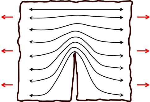
Most minerals are crystalline materials in which the atoms are regularly arranged in three-dimensional arrays. The configuration of atoms is determined by the size and types of physical and chemical bonds holding them together. In the crystalline lattice of minerals, these inter-atomic bonds are effective only over small distances, and can be broken if extended by a tensile stress. Such stresses may be generated by tensile or compressive loading (Figure 5.1).

Figure 5.1 Strain of a crystal lattice resulting from tensile or compressive stresses.

Even when rocks are uniformly loaded, the internal stresses are not evenly distributed, as the rock consists of a variety of minerals dispersed as grains of various sizes. The distribution of stress depends upon the mechanical properties of the individual minerals, but more importantly upon the presence of cracks or flaws in the matrix, which act as sites for stress concentration (Figure 5.2).

Figure 5.2 Stress concentration at a crack tip.

It has been shown (Inglis, 1913) that the increase in stress at such a site is proportional to the square root of the crack length perpendicular to the stress direction. Therefore, there is a critical value for the crack length at any particular level of stress at which the increased stress level at the crack tip is sufficient to break the atomic bond at that point. Such rupture of the bond will increase the crack length, thus increasing the stress concentration and causing a rapid propagation of the crack through the matrix, thus causing fracture.

Although the theories of comminution assume that the material is brittle, crystals can store energy without breaking, and release this energy when the stress is removed. Such behavior is known as elastic. When fracture does occur, some of the stored energy is transformed into free surface energy, which is the potential energy of atoms at the newly produced surfaces. Due to this increase in surface energy, newly formed surfaces are often more chemically active, being more amenable to the action of flotation reagents, for example. They also oxidize more readily in the case of sulfide minerals.

Griffith (1921) showed that materials fail by crack propagation when this is energetically feasible, that is, when the energy released by relaxing the strain energy is greater than the energy of the new surface produced. Brittle materials relieve the strain energy mainly by crack propagation, whereas “tough” materials can relax strain energy without crack propagation by the mechanism of plastic flow, where the atoms or molecules slide over each other and energy is consumed in distorting the shape of the material. Crack propagation can also be inhibited by encounters with other cracks or by meeting crystal boundaries. Fine-grained rocks, such as taconites, are therefore usually tougher than coarse-grained rocks.

The energy required for comminution is reduced in the presence of water, and can be further reduced by chemical additives which adsorb onto the solid (Hartley et al., 1978). This may be due to the lowering of the surface energy on adsorption providing that the surfactant can penetrate into a crack and reduce the bond strength at the crack tip before rupture.

Natural particles are irregularly shaped, and loading is not uniform but is achieved through points, or small areas, of contact. Breakage is achieved mainly by crushing, impact and attrition, and all three modes of fracture (compressive, tensile and shear) can be discerned depending on the rock mechanics and the type of loading, that is, the comminution device.

When an irregular particle is broken by compression, or crushing, the products fall into two distinct size ranges—coarse particles resulting from the induced tensile failure, and fines from compressive failure near the points of loading, or by shear at projections (Figure 5.3). The amount of fines produced can be reduced by minimizing the area of loading, and this is often done in compressive crushing machines by using corrugated crushing surfaces (Partridge, 1978; Chapter 6).

In impact breakage, due to the rapid loading, a particle experiences a higher average stress while undergoing more strain than is necessary to achieve simple fracture, and tends to break apart rapidly, mainly by tensile failure. The products from impact breakage when failure occurs are typically linear when cumulative finer is plotted in log–log space (e.g., Figure 4.7). If impact energy is lower than the yield stress, fracture may not occur but chipping, where edges are broken away, does.

Attrition or abrasion is not strictly a breakage event but rather a surface phenomenon where shear stress causes material to abrade off. It produces much fine material, and may be undesirable depending on the comminution stage and industry sector. Attrition occurs due to particle–particle interaction and in stirred mills due to media–particle interaction as well; attrition seems to be the main mechanism in stirred mills.

5.3 Comminution Modeling

Models for comminution processes fall into the three categories: empirical, phenomenological, and fundamental. Under empirical are the energy-based models. These are used in preliminary and detailed design, for assessing comminution efficiency, and for geometallurgy (distributing hardness data into mine block models, Chapter 17). Phenomenological models include population balance models, which have some underlying principles but with parameters fitted by calibration for given comminution devices. They are widely used in unit and circuit simulators. Lastly, the fundamental models include those based on discrete element method (DEM), computational fluid dynamics (CFD) and, some would argue, statistical physics (Martins and Radziszewski, 2014). They are computationally intensive, used for design and optimization of specific components of crushers, tumbling mills, and material handling systems.

5.3.1 Energy-based Comminution Models

This family of models is the oldest of the comminution models and they continue to find widespread use (Morrell, 2014a). Energy-based models assume a relationship between energy input of the comminution device and the resultant effective particle size of the product. Many rely on the feed and product size distributions being self-similar; that is, parallel when cumulative finer is plotted in log-log space (Chapter 4). The energy input is for net power, that is, after correcting for motor efficiency and drive train mechanical losses. Typically, energy is measured as kWh t⁻¹ or Joules, depending on the model.

The most familiar general energy-based comminution equation is that first presented by Walker et al. (1937). In differential form it is:

$d E = - K x^{- n} d x$ $d E = - K x^{- n} d x$ (5.1a)

(5.1a)

where dE is the increment in energy to effect an incremental decrease dx in particle size x, and n and K are constants (K also converts units). In integral form it is:

$E = - K \int_{F}^{P} x^{- n} d x$ $E = - K \int_{F}^{P} x^{- n} d x$ (5.1b)

(5.1b)

where F and P are some measure of feed and product particle size (usually a diameter). Letting n=2, 1 or 3/2 gives the “three comminution laws” due to Von Rittinger, Kick, and Bond.

The oldest theory, Von Rittinger (1867), stated that the energy consumed in size reduction is proportional to the area of new surface produced. The surface area of a known weight of particles of uniform diameter is inversely proportional to the diameter, hence Von Rittinger’s law equates to:

$E_{V R} = K (\frac{1}{P} - \frac{1}{F})$ $E_{V R} = K (\frac{1}{P} - \frac{1}{F})$ (5.2)

(5.2)

which is the solution of Eq. (5.1b) for n=2.

The second oldest theory, Kick (1885), stated that the energy required is proportional to the reduction in volume of the particles. Solving Eq. (5.1b) for n=1 gives one form of the Kick equation:

$E_{K} = K (\ln \frac{F}{P})$ $E_{K} = K (\ln \frac{F}{P})$ (5.3)

(5.3)

where F/P is the reduction ratio. Kick’s theory is that energy requirement depends only the reduction ratio, and not on the original size of the particles.

As Lynch and Rowland (2005) note, the means to make measurements of energy and size necessary to validate the Von Rittinger and Kick models did not exist until the middle of the twentieth century when electrical motors and precision laboratory instruments became available. The literature from this period includes work by a group at the Allis Chalmers Company who were trying to calibrate Von Rittinger’s equation to industrial rod mills (Bond and Maxson, 1938; Myers et al., 1947).

Often referred to as the “third theory”, Bond (1952) stated that the energy input is proportional to the new crack tip length produced in particle breakage. Bond redefined his “theory” to rather be an empirical relationship in a near-final treatise (Bond, 1985). The equation is commonly written as:

$W = 10 \times W i (\frac{1}{\sqrt{P_{80}}} - \frac{1}{\sqrt{F_{80}}})$ $W = 10 \times W i (\frac{1}{\sqrt{P_{80}}} - \frac{1}{\sqrt{F_{80}}})$ (5.4)

(5.4)

where W is the energy input (work) in kilowatt hours per metric ton (or per short ton in Bond’s original publications), Wi is the work index (or Bond work index) in kilowatt hours per metric ton, and P₈₀ and F₈₀ are the 80% product and feed sizes, in micrometers.

Solving Eq. (5.1b) for n=3/2 gives the same form as Eq. (5.4) with the constant 2 K ahead of the bracket. In effect the 2 K is replaced by (10×Wi), which is convenient because Wi becomes equal to W in the case of grinding from a theoretical infinite feed size to 80% passing 100 µm. The Bond model remains the most widely used, at least for the “conventional” comminution equipment in use at the time Bond developed the model and calibrated it against industrial data. It is one reason that the 80% passing size became the common single point metric (“mean”) of a particle size distribution.

A modification of Eq. (5.1a,b) was proposed by Hukki (1962), namely substituting n by a function of particle size, f(x). This provoked debate over the size range that the three established models applied to. What can be agreed is that all the models predict that energy consumption will increase as product particle size (i.e., P) decreases. Typical specific energy values (in kWh t⁻¹) are (Morrell, 2014b): primary crushing (i.e., 1000–100 mm), 0.1–0.15; secondary crushing (100-10 mm), 1–1.2; coarse grinding (10-1 mm), 3–3.5; and fine grinding (1-0.1 mm), 10.

Fine grinding tests are sometimes expressed as a signature plot (He et al., 2010), which is an experimentally fitted version of Eq. (5.1a,b) with n=f(x). A laboratory test using a fine grinding mill is conducted where the energy consumption is carefully measured and a slurry sample is extracted periodically to determine the 80% passing size. The energy-time relationship versus size is then plotted and fitted to give (in terms of Eq. (5.1a,b)) a coefficient K and a value for the exponent f (x).

Recently, Morrell (2004a) proposed an energy-based model of size reduction that also incorporates particle size dependence:

$d E = - M g {(x)}^{- f (x)} d x$ $d E = - M g {(x)}^{- f (x)} d x$ (5.5)

(5.5)

where g(x) is a function describing the variation in breakage properties with particle size, and M a constant related to the breakage properties of the material.

The problem that occurs when trying to solve Eq. (5.5) is the variable nature of the function g(x). A pragmatic approach was to assume M is a constant over the normal range of particle sizes treated in the comminution device and leave the variation in size-by-size hardness to be taken up by f(x). Morrell (2009) gives the following:

$W = M_{i} 4 (P^{f (P)} - F^{f (F)})$ $W = M_{i} 4 (P^{f (P)} - F^{f (F)})$ (5.6)

(5.6)

where M_i is the work index parameter related to the breakage property of an ore and the type of comminution machine, W is the specific comminution energy (kWh t⁻¹), P and F are the product and feed 80% passing size (μm), and f(x) is given by (Morrell, 2006):

$f (x) = (0.295 + \frac{x}{10^{6}})$ $f (x) = (0.295 + \frac{x}{10^{6}})$ (5.7)

(5.7)

The parameter M_i takes on different values depending on the comminution machine: M_ia for primary tumbling mills (AG/SAG mills) that applies above 750 μm; M_ib for secondary tumbling mills (e.g., ball mills) that applies below 750 μm; M_ic for conventional crushers; and M_ih for HPGRs. The values for M_ia, M_ic, and M_ih were developed using the SMC Test® combined with a database of operating comminution circuits. A variation of the Bond laboratory ball work index test was used to determine values of M_ib. This is similar to the approach Bond used in relating laboratory results to full scale machines. The methodology continues to be refined as the database expands (Morrell, 2010).

Morrell (2009) gave a worked example comparing the energy requirements for three candidate circuits to illustrate the calculations. Taking just the example for the fine particle tumbling mill serves that purpose here (Example 5.1).

Example 5.1

An SMC Test® and Bond ball mill work index test (with closing screen 150 μm) were performed on an ore sample with the following results:

$M_{i a} = 19.4 kWh t^{- 1}; M_{i c} = 7.2 {kWh}^{- 1}; M_{i h} = 13.9 {kWh}^{- 1}; M_{i b} = 18.8 kWh t^{- 1} .$ $M_{i a} = 19.4 kWh t^{- 1}; M_{i c} = 7.2 {kWh}^{- 1}; M_{i h} = 13.9 {kWh}^{- 1}; M_{i b} = 18.8 kWh t^{- 1} .$

Calculate the specific grinding energy for the fine particle tumbling mill to give a product P₈₀ of 106 μm.

Solution

From the M_i data the relevant value is M_ib=18.8 kWh t⁻¹. Noting it is fine grinding then the feed F₈₀ is taken as 750 μm. Combining Eqs. (5.6) and (5.7) and substituting the values:

$\begin{array}{l} W & = 18.8 \times 4 \times (106^{- (0.295 + 750 / 1, 000, 000)} - 750^{- (0.295 + 750 / 1, 000, 000)}) \\ = 8.4 (k W h t^{- 1}) \end{array}$ $\begin{array}{l} W & = 18.8 \times 4 \times (106^{- (0.295 + 750 / 1, 000, 000)} - 750^{- (0.295 + 750 / 1, 000, 000)}) \\ = 8.4 (k W h t^{- 1}) \end{array}$

5.3.2 Breakage Characterization

Using the energy-based models requires estimates of parameters that relate to the ore, variously expressed as hardness, grindability, or resistance to breakage. This has given rise to a series of procedures, summarized by Mosher and Bigg (2002) and Morrell (2014a).

Bond Tests

The most widely used parameter to measure ore hardness is the Bond work index Wi. Calculations involving Bond’s work index are generally divided into steps with a different Wi determination for each size class. The low energy crushing work index laboratory test is conducted on ore specimens larger than 50 mm, determining the crushing work index (Wi_C, CWi or IWi (impact work index)). The rod mill work index laboratory test is conducted by grinding an ore sample prepared to 80% passing 12.7 mm (½ inch, the original test being developed in imperial units) to a product size of approximately 1 mm (in the original and still the standard, 14 mesh; see Chapter 4 for definition of mesh), thus determining the rod mill work index (Wi_R or RWi). The ball mill work index laboratory test is conducted by grinding an ore sample prepared to 100% passing 3.36 mm (6 mesh) to product size in the range of 45–150 µm (325-100 mesh), thus determining the ball mill work index (Wi_B or BWi). The work index calculations across a narrow size range are conducted using the appropriate laboratory work index determination for the material size of interest, or by chaining individual work index calculations using multiple laboratory work index determinations across a wide range of particle size.

To give a sense of the magnitude, Table 5.1 lists Bond work indices for a selection of materials. For preliminary design purposes such reference data are of some guide but measured values are required at the more advanced design stage.

Table 5.1

Selection of Bond Work Indices (kWh t⁻¹)

Material	Work Index	Material	Work Index
Barite	4.73	Fluorspar	8.91
Bauxite	8.78	Granite	15.13
Coal	13.00	Graphite	43.56
Dolomite	11.27	Limestone	12.74
Emery	56.70	Quartzite	9.58
Ferro-silicon	10.01	Quartz	13.57

A major use of the Bond model is to select the size of tumbling mill for a given duty. (An example calculation is given in Chapter 7.) A variety of correction factors (EF) have been developed to adapt the Bond formula to situations not included in the original calibration set and to account for relative efficiency differences in certain comminution machines (Rowland, 1988). Most relevant are the EF₄ factor for coarse feed and the EF₅ factor for fine grinding that attempt to compensate for sizes ranges beyond the bulk of the original calibration data set (Bond, 1985).

The standard Bond tumbling mill tests are time-consuming, requiring locked-cycle testing. Smith and Lee (1968) used batch-type tests to arrive at the work index; however, the grindability of highly heterogeneous ores cannot be well reproduced by batch testing.

Berry and Bruce (1966) developed a comparative method of determining the hardness of an ore. The method requires the use of a reference ore of known work index. The reference ore is ground for a certain time (T) in a laboratory tumbling mill and an identical weight of the test ore is then ground for the same time. Since the power input to the mill is constant (P), the energy input (E=P×T) is the same for both reference and test ore. If r is the reference ore and t the ore under test, then we can write from Bond’s Eq. (5.4):

$\begin{array}{l} W_{r} = W_{t} = W i_{r} [\frac{10}{\sqrt{P_{80 r}}} - \frac{10}{\sqrt{F_{80 r}}}] = W i_{t} [\frac{10}{\sqrt{P_{80 t}}} - \frac{10}{\sqrt{F_{80 t}}}] \end{array}$ $\begin{array}{l} W_{r} = W_{t} = W i_{r} [\frac{10}{\sqrt{P_{80 r}}} - \frac{10}{\sqrt{F_{80 r}}}] = W i_{t} [\frac{10}{\sqrt{P_{80 t}}} - \frac{10}{\sqrt{F_{80 t}}}] \end{array}$

Therefore:

$\begin{array}{l} W i_{t} = W i_{r} \frac{[\frac{10}{\sqrt{P_{80 r}}} - \frac{10}{\sqrt{F_{80 r}}}]}{[\frac{10}{\sqrt{P_{80 t}}} - \frac{10}{\sqrt{F_{80 t}}}]} \end{array}$ $\begin{array}{l} W i_{t} = W i_{r} \frac{[\frac{10}{\sqrt{P_{80 r}}} - \frac{10}{\sqrt{F_{80 r}}}]}{[\frac{10}{\sqrt{P_{80 t}}} - \frac{10}{\sqrt{F_{80 t}}}]} \end{array}$ (5.8)

(5.8)

Reasonable values for the work indices are obtained by this method as long as the reference and test ores are ground to about the same product size distribution.

Work indices have been obtained from grindability tests on different sizes of several types of equipment, using identical feed materials (Lowrison, 1974). The values of work indices obtained are indications of the efficiencies of the machines. Thus, the equipment having the highest indices, and hence the largest energy consumers, are found to be jaw and gyratory crushers and tumbling mills; intermediate consumers are impact crushers and vibration mills, and roll crushers are the smallest consumers. The smallest consumers of energy are those machines that apply a steady, continuous, compressive stress on the material.

A class of comminution equipment that does not conform to the assumption that the particle size distributions of a feed and product stream are self-similar includes autogenous mills (AG), semi-autogenous (SAG) mills and high pressure grinding rolls (HPGR). Modeling these machines with energy-based methods requires either recalibrating equations (in the case of the Bond series) or developing entirely new tests that are not confused by the non-standard particle size distributions.

Drop Weight Tests

In contrast to the Bond tests which yield a single work index value, drop weight tests are designed to produce more detailed information on the size distributions produced on breaking rocks and their relationship to input energy. This was required for comminution circuit simulations, one of the aims being the prediction of size distribution from comminution units to link to other units, such as classifiers. The JK Drop-weight Test, for example, is linked to the JK comminution models (Morrell, 2014b).

The JK Drop-weight Test is conducted on single-size particles ranging from −63+53 mm to −16+13.2 mm. Each size class is broken at three input energies and the progeny particles sized. From the size distribution the fraction less than 1/10th the original size is determined, the t₁₀. The t₁₀ is related to the associated input specific energy (Ecs, kWh t⁻¹) by the following:

$t_{10} = A [1 - e^{(- b . E c s)}]$ $t_{10} = A [1 - e^{(- b . E c s)}]$ (5.9)

(5.9)

where A and b are dependent on the ore properties (type, size, etc.). The product A×b can be correlated with other comminution system variables: a high A×b, for example, indicates material easy to break and corresponds to a low work index, Wi. The t₁₀ can be related to other t_n values. This approach is described in detail by Napier-Munn et al. (1996).

A drawback of the drop-weight test is that usually over 60 kg of rock are required for a single test. This problem is addressed with the introduction of the SMC Test^R, noted earlier, which reduces the amount of sample required (Morrell, 2004b).

MacPherson Test

Developed by Art MacPherson while at Aerofall Mills Ltd., it uses a 450 mm dry air-swept SAG mill with an 8% ball charge. The test is run in closed circuit to steady state. At completion, the particle size distribution (PSD) is measured. Based on the PSD of feed and product and the measured power input, the autogenous work index (AWi) is determined. Two drawbacks of the test are: it is restricted to particles finer than 32 mm, and due to the low number of high energy impacts a correction for hard ores is required (Mosher and Bigg, 2002).

SPI and SGI Tests

The SPI™ (SAG Power Index, trademark of SGS Mineral Services and invented by John Starkey) and the generic SGI (SAG Grindability Index) tests are dry batch tests commonly used for ore variability characterization in SAG milling circuits. The main differences between the SPI and the SGI are: 1) sample prep for the test feed is different; 2) the SGI is run progressively with fixed timing. The two, largely interchangeable, batch tests are conducted in a 30.5 cm diameter by 10.2 cm long grinding mill charged with 5 kg of steel balls. Two kilograms of sample are crushed to 100% minus 1.9 cm and 80% minus 1.3 cm and placed in the mill. The test is run until the sample is reduced to 80% minus 1.7 mm. The test result is M, the time (in minutes) required to reach a P₈₀ of 1.7 mm (Starkey and Dobby, 1996). This time is used to calculate the SAG mill specific energy, E_SAG, either via the proprietary SPI equation (Kosick and Bennett, 1999) or a published SGI equation (Amelunxen et al., 2014):

$E_{S A G} = K {(\frac{M}{\sqrt{p_{80}}})}^{n} f_{S A G}$ $E_{S A G} = K {(\frac{M}{\sqrt{p_{80}}})}^{n} f_{S A G}$ (5.10)

(5.10)

where K and n are empirical factors, and f_SAG incorporates a series of calculations that estimate the influence of factors such as pebble crusher recycle load (Chapter 6), ball load, and feed size distribution. Amelunxen et al. (2014) published a set of parameters (calibrated mostly from porphyry ores in the Americas) for the SGI equation where K=5.9, n=0.55 and f_SAG=1.0 for a circuit without pebble crushing or f_SAG=0.85 for a circuit with pebble crushing.

SAGDesign Test

The Standard Autogenous Grinding Design (SAGDesign) test measures macro and micro ore hardness by means of a SAG mill test and a standard Bond ball mill work index test on SAG ground ore. Ore feed is prepared from a minimum of 10 kg of split diamond drill core samples by stage crushing the ore in a jaw crusher to 80% product passing 19 mm. The SAG test reproduces commercial SAG mill grinding conditions on 4.5 liter of ore and determines the SAG mill specific pinion energy needed to grind ore from 80% passing 152 mm to 80% passing 1.7 mm, herein referred to as macro ore hardness. The SAG mill product is then crushed to 100% passing 3.35 mm and is subjected to a standard Bond ball mill work index (S_d-BWi) grinding test to provide the total pinion energy at the specified grind size for mill design purposes. A calibration equation is used to convert the test result (total number of revolutions to reach the endpoint and the initial mass of feed ore) to the pinion energy. The SAGDesign test has been abbreviated for the needs of geometallurgy, that is, measuring the ore variability in a deposit (Brissette et al., 2014).

Bond-based AG/SAG Models

Several authors have developed autogenous and semiautogenous grinding models that are re-calibrated versions of Bond equations (e.g., Barratt, 1979; Sherman, 2011; Lane et al., 2013). These methods typically partition SAG breakage into ranges of particle sizes where one or another of the Bond work index values is used, the sum of which is then multiplied by empirical adjustment factors to give an estimate of the SAG mill (or SAG-ball mill circuit) specific energy consumption. A detailed example of a Bond-type SAG circuit sizing calculation is provided by Doll (2013).

The validity of the Bond method has been questioned in the case of coarser particle sizes in SAG milling (Millard, 2002). Laboratory testing of rocks at different sizes frequently indicates material reporting harder (higher) crushing work index values at coarser sizes. If the model is valid, then the only way this is possible is if the defects (fractures) where a rock breaks are eliminated at larger sizes, which is plainly not possible. Fortunately, Bond-based models tend to not be sensitive to coarse sized material due to the (F₈₀)^−½ term being small in relation to the (P₈₀)^−½ term.

5.3.3 Population Balance Models

The energy-based models, such as the Bond model, do not predict the complete product size distribution, only the 80% passing size, nor do they predict the effect of operating variables on mill circulating load, nor classification performance. The complete size distribution is required in order to simulate the behavior of the product in ancillary equipment such as screens and classifiers, and for this reason population balance models are used in the design, optimization and control of grinding circuits (Napier-Munn et al., 1996).

Population balance—or mass-size balance—describes a family of modeling techniques that involve tracking and manipulating whole (or partial) particle size distributions as they proceed through the comminution process (or, indeed, any mineral processing unit). These techniques allow grinding circuits to be simulated without the assumption that all particle size distributions have a “normal” shape (as in many energy-based models), but at a cost of being more computationally intensive and requiring more model configuration parameters.

There are various commercially available programs that perform this style of modeling (e.g., USIMpac, JK SimMet, and Moly-Cop Tools). A range of case studies can be found in the literature, covering both design and optimization of grinding circuits. Examples include Richardson (1990), Lynch and Morrell (1992), McGhee et al. (2001), and Dunne et al. (2001).

The general equation describing any comminution device is (Napier-Munn et al., 1996; King, 2012):

$p_{i} = T_{i} f_{i}$ $p_{i} = T_{i} f_{i}$ (5.11)

(5.11)

where p_i, f_i are the fraction in size class i in product and feed, respectively, and T_i is some transfer function. The task is to determine T_i.

This modeling approach is most often applied to tumbling mills. The starting assumption is that the rate of disappearance (rate of breakage) of mass of size class i is proportional to the mass of that size fraction in the mill at time t, f_i(t), that is, a first-order kinetics model:

$\frac{d f_{i} (t)}{d t} = - S_{i} f_{i} (t)$ $\frac{d f_{i} (t)}{d t} = - S_{i} f_{i} (t)$ (5.12)

(5.12)

where S_i is the specific rate of breakage (or selection) parameter of size class i. By convention, the size classes are numbered 1 to n, from coarsest to finest (with n+1 being the pan fraction in a typical sieve sizing method).

To complete the balance on any size class, the breakage into and out of that class is required. This introduces a second parameter, the breakage (or breakage appearance) parameter, B:

$\frac{d f_{i} (t)}{d t} = \sum_{j = 1}^{i - 1} B_{i j} S_{j} f_{j} (t) - S_{i} f_{i} (t)$ $\frac{d f_{i} (t)}{d t} = \sum_{j = 1}^{i - 1} B_{i j} S_{j} f_{j} (t) - S_{i} f_{i} (t)$ (5.13)

(5.13)

where B_ij describes the fraction of size j (j<i) that reports to size i. If we apply the balance around a single size class then the solution to Eq. (5.13) is (dropping the t):

$\begin{array}{l} Product out = Feed in + Breakage in - Breakage out \\ p_{i} = f_{i} + \sum_{j = 1}^{i - 1} B_{i j} S_{j} f_{i} - S_{i} f_{i} or \sum_{j = 1}^{i - 1} B_{i j} S_{j} f + (1 - S) f_{i} \end{array}$ $\begin{array}{l} Product out = Feed in + Breakage in - Breakage out \\ p_{i} = f_{i} + \sum_{j = 1}^{i - 1} B_{i j} S_{j} f_{i} - S_{i} f_{i} or \sum_{j = 1}^{i - 1} B_{i j} S_{j} f + (1 - S) f_{i} \end{array}$ (5.14)

(5.14)

Provided we know the B and S parameters as a function of size, we can predict the product size distribution.

The simplest way to test the model is to consider the rate of disappearance of the top size class. Writing Eq. (5.12) for size class (sieve) 1 and assuming all particles have the same residence time (as in batch grinding) we derive:

$\ln (\frac{f_{1} (t)}{f_{1} (0)}) = - S_{1} t$ $\ln (\frac{f_{1} (t)}{f_{1} (0)}) = - S_{1} t$ (5.15)

(5.15)

where f₁(0) and f₁(t) are the initial weight and weight retained after t grind time, and S₁ is the rate of breakage parameter for size class 1. Table 5.2 and Figure 5.4 show the result of a laboratory batch ball-mill grinding test on a sample of Pb-Zn ore taken from a ball mill feed. Figure 5.4 shows that the rate of disappearance of “coarse” material does obey the first order rate model; the slope is S and we note that S increases with increasing particle size (usually to a maximum depending on factors such as media size to particle size). The equation could have been written in terms of fine material: the rate of appearance of fines would also follow the first-order model. This is a common finding for batch tests (Austin et al., 1984) but first order appearance of fines has also long been recognized in continuous milling (Dorr and Anable, 1934).

Table 5.2

Cumulative Mass Retained as a Function of Time (%)

Size (µm)	Time (min)
Size (µm)	0	2	4	6	8	10	12
600	13.12	3.83	1.66	0.70	0.33	0.15	0.10
300	29.99	13.36	5.49	2.11	0.78	0.31	0.16
150	52.05	35.98	24.24	15.64	8.64	5.05	2.81
75	77.10	66.30	56.71	48.37	40.16	33.05	27.60
37	87.62	81.52	75.02	69.88	64.49	59.97	55.69

Figure 5.4 Test of first order grinding kinetics, the “disappearance plot” (Eq. (5.15)).

Figure 5.5 shows the general relationship for the rate of breakage parameter as a function of particle size for ball milling and SAG milling. The maximum is related to the ball size to particle size ratio passing through an optimum (at too large a particle size the balls are too small for effective breakage). The minimum is related to the “critical size” observed in AG/SAG milling where particles of this size self-break slowly and build up in the mill requiring extraction and crushing to eliminate (Chapters 6 and 7).

Figure 5.5 General result for specific rate of breakage as a function of particle size.

The model (Eq. (5.14)) can be combined with information on material transport, measured by the distribution of residence times in the mill, and mill discharge characteristics to provide a description of open-circuit grinding, which can be coupled with information concerning the classifier to produce closed-circuit grinding conditions (Napier-Munn et al., 1996). A simplification for closed circuit ball mill grinding is that transport can be approximated by plug flow (Furuya et al., 1971). In that case Eq. (5.15), the solution for batch grinding and hence also plug flow, applies. (See Chapter 12 for more discussion on material transport.) These models can only realize their full potential, however, if there are accurate methods of estimating the B and S model parameters (or functions). The complexity of the breakage environment in a tumbling mill precludes the calculation of these values from first principles, so that successful application depends on the development of techniques for the calibration of model parameters to experimental data. There are methods to estimate the selection and breakage functions simultaneously (e.g., Rajamani and Herbst, 1984). Commercial simulators often use a default breakage function, which is a drawback. Refinements to determine S and B continue to evolve (Shi and Xie, 2015).

Experimental characterization of the properties of heterogeneous ores is a challenge in population-type models. Although breakage characteristics for homogeneous materials can be determined on a small scale and used to predict large-scale performance, it is more difficult to predict the behavior of mixtures of two or more components. Furthermore, the relationship of material size reduction to subsequent processing is even more difficult to predict (e.g., using the output of population balance comminution models to predict flotation characteristics) due to the complexities of mineral release (liberation). Work has advanced on the development of grinding models that include mineral liberation in the size-reduction description (Choi et al., 1988; Herbst et al., 1988). An entropy-based multiphase approach, which models particles individually rather than the standard approach of using composite classes, is seen as an advance (Gay, 2004). The development of liberation models is essential if simulation of integrated plants is to be realized.

Linking to Energy

The mass-size balance models as written above are in the time-domain. To be more practical they need to be converted to the energy-domain. One way is by arguing that the specific rate of breakage parameter is proportional to the net specific power input to the mill charge (Herbst and Fuerstenau, 1980; King, 2012). For a batch mill this becomes:

$S_{i} = S_{i}^{E} \frac{P}{M}$ $S_{i} = S_{i}^{E} \frac{P}{M}$ (5.16)

(5.16)

where $S_{i}^{E}$ $S_{i}^{E}$ is the energy-specific rate of breakage parameter, P the net power drawn by the mill, and M the mass of charge in the mill excluding grinding media (i.e., just the ore). The energy-specific breakage rate is commonly given in t kWh⁻¹. For a continuous mill, the relationship is:

$S_{i} τ = S_{i}^{E} \frac{P}{F}$ $S_{i} τ = S_{i}^{E} \frac{P}{F}$ (5.17)

(5.17)

where τ is the mean retention time, and F the solids mass flow rate through the mill. Assuming plug flow, Eq. (5.17) can be substituted into Eq. (5.15) to apply to a grinding mill in closed circuit (where t=τ).

Simplified Grinding Model

The result in Figure 5.5 suggests a simplified approach to grinding models by basing on disappearance of “coarse” without reference to where the products end up, that is, eliminating the B function. Given that the coarse fraction is determined by cumulating the data above a given size (see Table 5.2), the S–parameter is no longer size discrete but on a cumulative basis. Thus, the model is also referred to as the cumulative-basis grinding model.

Finch and Ramirez-Castro (1981) adopted the cumulative basis model in order to extend the grinding model to mineral classes, which otherwise would require the estimation of the B function for these classes, making an already difficult task essentially insurmountable. Applied to a Pb-Zn ore, they found that mineral grinding rates were similar but classification was highly dependent on mineral density, which dominated the mineral size distributions in the ball mill-cyclone circuit (see also Chapter 9). Hinde and Kalala (2009) used the cumulative-basis model for tumbling mills, stirred mills and HPGRs in assessing competing circuit arrangements. They converted to the energy-domain by adapting the approach of Herbst and Fuerstenau (1980) (Eq. (5.16)) and confirmed the model in batch grinding tests. Jankovic and Valery (2013), in essence, used the cumulative-basis (or “coarse disappearance”) model in assessing closed circuit ball mill operation.

5.3.4 Fundamental Models

Use of Discrete Element Modeling (DEM) and Computational Fluid Dynamics (CFD), while becoming routine in modeling many unit operations in mineral processing (Chapter 17), has arguably been most widely applied to comminution units. The computationally-intensive technique combines detailed physical models to describe the motion of balls, rocks, and slurry and attendant breakage of particles as they are influenced by moving liners/lifters and grates. Powell and Morrison (2007) make the case that the future of comminution modeling must include these advanced techniques that the ever-increasing computational power brings into reach.

These advanced modeling techniques applied to tumbling mills are leading to improved understanding of charge dynamics, and to improved designs of mill internals. There is potential to reduce downtime and increase the efficient use of energy. The approach has been shown to reliably model breakage in tumbling mills (Carvalho and Tavares, 2010), and is in common use simulating breakage in crushers (Quist and Evertsson, 2010; Kiangi et al., 2012). Applied to stirred mills it has helped identify the importance of shear in size reduction (Radziszewski, 2013a). Incorporating slurry properties, moving to simulation of continuous operation (simulations are currently batch and the introduction of feed is a disturbance to charge motion), and direct prediction of particle breakage are some of the areas of active research.

One of the features of three-dimensional DEM simulation is the cutaway images of particle motion in the mill, an example being in Figure 5.6 for a 1.8 m diameter pilot SAG mill. Radziszewski and Allen (2014) provide a series of images of charge motion in stirred mills.

Figure 5.6 Example of ball and particle motion in a slice of a pilot SAG mill using three-dimensional DEM simulation (Courtesy CSIRO (Dr. Paul Cleary)).

Validation of the predictions made by DEM/CFD models is critical to verifying the simulations. Visual inspection through a transparent end wall is commonly used (e.g., Maleki-Moghaddam et al., 2013). Figure 5.7 shows a good agreement between simulation and experiment for charge motion for a scaled-down SAG mill. Positron Emission Particle Tracking (PEPT, Chapter 17) is a powerful non-invasive tool for validation but is restricted by the size of the scanner to relatively small test units. Acoustic monitoring of industrial-scale units provides another non-invasive opportunity to test model predictions, for example, detecting where balls strike the shell (Pax, 2012).

Figure 5.7 Comparison of three-dimensional DEM with experiment for 75% critical speed, scale model 0.6 m diameter SAG mill (Courtesy CSIRO (Dr. Paul Cleary)).

5.4 Comminution Efficiency

Comminution consumes the largest part of the energy used in mining operations, from 30 to 70% (Radziszewski, 2013b; Nadolski et al., 2014). This has consequently drawn most of the sustainability initiatives designed to reduce energy consumption in mining, including, for example, the establishment of CEEC (Coalition for Eco-efficient Comminution, www.ceecthefuture.org) and GMSG (Global Mining Standards Guidelines Group, www.globalminingstandards.org).

One approach is to ask if all the ore needs fine grinding, where the bulk of the energy is consumed. Certainly in the case of low grade ores, much of the gangue can be liberated at quite coarse size and its further size reduction would represent inefficient expenditure of comminution energy (Chapter 1). This provides an opportunity for ore sorting, for example (Chapter 14). Lessard et al. (2014) provide case studies showing the impact on comminution energy of including ore sorting on crusher products ahead of grinding. Similar in objective, the development of coarse particle flotation technologies (Chapter 12) aims to reduce the mass of material sent to the fine grinding (liberation) stage.

This still leaves the question of how efficiently the energy is used in comminution. It is common experience that significant heat is generated in grinding (in particular) and can be considered a loss in efficiency. However, it may be that heat is an inevitable consequence of breakage. Capturing the heat could even be construed as a benefit (Radziszewski, 2013b).

A fundamental approach to assessing energy efficiency is to compare input energy relative to the energy associated with the new surface created. This increase in surface energy is calculated by multiplying the area of new surface created (m²) by the surface tension expressed as an energy (J m⁻²). On this basis, efficiency is calculated to be as little as 1% (Lowrison, 1974). This may not be an entirely fair basis to evaluate as we suspect that some input energy goes into deforming particles and creating micro-cracks (without breakage) and that the new surface created is more energetic than the original surface, meaning the surface tension value may be underestimated. In addition, both these factors may provide side-benefits of comminution. Rather than this comparison as a basis, other measures use a comparison against a “standard.”

Possible Standards

Single particle slow compressive loading is considered about the most energy efficient way to comminute. Comparing to this basis, Fuerstenau and Abouzeid (2002) found that ball milling quartz was about 15% energy efficient. From theoretical reasoning, Tromans (2008) estimated the energy associated with breakage by slow compression and showed that relative to this value the efficiency of creating new surface area could be as high as 26%, depending on the mineral.

Nadolski et al. (2014) propose an “energy benchmarking” measure based on single particle breakage. A methodology derived from the JK Drop-weight Test is used to determine the limiting energy required for breakage, termed the “essential energy.” They derive a comminution benchmark energy factor (BEF) by dividing actual energy consumed in the comminution machine by the essential energy. They make the point that the method is independent of the type of equipment, and can be used to include energy associated with material transport as well to assess competing circuit designs.

A standard already in use is the Bond work index against which the operating work index can be compared.

Operating Work Index Wi_O

This is obtained for a comminution device using Eq. (5.4), by measuring W (the specific energy being used, kWh t⁻¹), F₈₀ and P₈₀ and solving for Wi as the operating work index, Wi_O. (Note that the value of W is the power applied to the pinion shaft of the mill. Motor input power thus has to be converted to power at the mill pinion shaft output by applying corrections for electrical and mechanical losses between the power measurement point and the shell of the mill.) The ratio of laboratory determined work index to operating work index, Wilab:Wi_O, is the measure of efficiency relative to the standard: for example, if Wilab:Wi_O <1, the unit or circuit is using more energy than predicted by the standard test, that is, it is less efficient than predicted. Values of Wilab:Wi_O obtained from specific units can be used to assess the effect of operating variables, such as mill speed, size of grinding media, type of liner, etc. Note, this means that the Bond work index has to be measured each time the comparison is to be made. An illustration of the use of this energy efficiency calculation is provided by Rowland and McIvor (2009) (Example 5.2).

Example 5.2

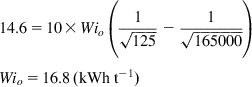
a. A survey of a SAG-ball mill circuit processing ore from primary crushing showed size reduction of circuit (SAG) feed F₈₀ of approximately 165,000 µm to flotation circuit feed (cyclone overflow) P₈₀ of 125 µm. The total specific energy input for the two milling stages was 14.6 kWh t⁻¹. Calculate the operating work index for the circuit.

b. Circuit feed samples taken at the same time were sent for Bond work index testing. The rod mill test gave RWilab of 14.5 kWh t⁻¹ and a ball mill work index BWilab of 13.8 kWh t⁻¹. Accepting that the rod mill work index applies to size reduction of the circuit feed down to the rod mill test product P₈₀ of 1050 µm and that the ball mill work index applies from this size to the circuit product size, calculate the standard Bond energy for the circuit.

c. Calculate the combined Wilab and the relative efficiency, Wilab:Wio. What do you conclude?

Solution

a. The appropriate form of Eq. (5.4) is:

$\begin{array}{l} 14.6 = 10 \times {W i}_{o} (\frac{1}{\sqrt{125}} - \frac{1}{\sqrt{165000}}) \\ {W i}_{o} = 16.8 (kWh t^{- 1}) \end{array}$ $\begin{array}{l} 14.6 = 10 \times {W i}_{o} (\frac{1}{\sqrt{125}} - \frac{1}{\sqrt{165000}}) \\ {W i}_{o} = 16.8 (kWh t^{- 1}) \end{array}$

b. Bond energy for both size reduction stages is:

From rod mill test:

$\begin{array}{l} W = 10 \times 14.5 (\frac{1}{\sqrt{1050}} - \frac{1}{\sqrt{165000}}) \\ W = 4.1 (kWh t^{- 1}) \end{array}$ $\begin{array}{l} W = 10 \times 14.5 (\frac{1}{\sqrt{1050}} - \frac{1}{\sqrt{165000}}) \\ W = 4.1 (kWh t^{- 1}) \end{array}$

From ball mill test:

$\begin{array}{l} W = 10 \times 13.8 (\frac{1}{\sqrt{125}} - \frac{1}{\sqrt{1050}}) \\ W = 8.1 (kWh t^{- 1}) \end{array}$ $\begin{array}{l} W = 10 \times 13.8 (\frac{1}{\sqrt{125}} - \frac{1}{\sqrt{1050}}) \\ W = 8.1 (kWh t^{- 1}) \end{array}$

Therefore predicted total is: W_T=12.2 kWh t⁻¹

c. The combined test work index for this ore, Wilab^C is given by:

$\begin{array}{l} 12.2 = 10 \times {Wilab}^{C} (\frac{1}{\sqrt{125}} - \frac{1}{\sqrt{165000}}) \\ {Wilab}^{C} = 14.0 (kWh t^{- 1}) \end{array}$ $\begin{array}{l} 12.2 = 10 \times {Wilab}^{C} (\frac{1}{\sqrt{125}} - \frac{1}{\sqrt{165000}}) \\ {Wilab}^{C} = 14.0 (kWh t^{- 1}) \end{array}$

and, thus:

$\frac{{Wilab}^{C}}{{W i}_{o}} = \frac{14.0}{16.8} = 0.83 (or 83 %)$ $\frac{{Wilab}^{C}}{{W i}_{o}} = \frac{14.0}{16.8} = 0.83 (or 83 %)$

This result indicates the circuit is only 83% efficient compared to that predicted by the Bond standard test.

The procedure has the virtue of simplicity and the use of well recognized formulae. Field studies have shown the ratio can vary as much as ±35% from unity (some circuits will operate at greater efficiency than the Bond energy predicts). Rowland and McIvor (2009) discuss some of the limitations of the method. They note that the size distributions from AG/SAG milling can be quite unlike those from rod and ball mills on which the technique originated; and, beyond giving a measure of efficiency, it does not provide any specific indication of the causes of inefficiency. In the case of ball mill-classifier circuits “functional performance analysis” does provide a tool to identify which of the two process units (or both) may be the source of inefficiency.

Functional Performance Analysis

McIvor (2006, 2014) has provided an intermediate level (i.e., between the simple lumped parameter work index of Bond, and the highly detailed computerized circuit modeling approach) to characterize ball mill-cyclone circuit performance.

Classification System Efficiency (CSE) is the percentage of “coarse” size (typically with reference to the P₈₀) material occupying the mill and can be calculated by taking the average of the percentage of coarse material in the mill feed and mill discharge. As this also represents the percentage of the mill energy expended on targeted, coarse size material, it is directly proportional to overall grinding circuit efficiency and production rate. Circuit performance can then be expressed in the Functional Performance Equation for ball milling circuits, which is derived as follows.

Define “fines” as any product size material, and “coarse” as that targeted to be further ground, the two typically differentiated by the circuit target P₈₀. For any grinding circuit, the production rate of new, product size material or fines (Production Rate of Fines, PRF) must equal the specific grinding rate of the coarse material (i.e., fine product generated per unit of energy applied to the coarse material) times the power applied to the coarse material:

$Circuit PRF = Power Applied to Coarse Material \times Specific Grinding Rate of Coarse Material$ $Circuit PRF = Power Applied to Coarse Material \times Specific Grinding Rate of Coarse Material$

The power applied to the coarse material is the total mill power times the fraction of coarse material in the mill, the latter already defined as CSE. Therefore:

$Circuit PRF = Mill Power \times CSE \times Specific Grinding Rate of Coarse Material$ $Circuit PRF = Mill Power \times CSE \times Specific Grinding Rate of Coarse Material$

A measure of the plant ball mill’s grinding efficiency is the ratio of the grinding rate of the coarse material in the plant ball mill compared to the grinding rate, or “grindability,” of the same coarse material (g rev⁻¹) as measured in a standardized test mill set up. That is:

$Mill Grinding Eff . = Specific Grinding Rate of Coarse Material / Material Grindability$ $Mill Grinding Eff . = Specific Grinding Rate of Coarse Material / Material Grindability$

Therefore, if we substitute for specific grinding rate of coarse in the previous equation, we have the Functional Performance Equation for ball milling circuits:

$Circuit PRF = Mill Power \times CSE \times Mill Grinding Efficiency \times Material Grindability$ $Circuit PRF = Mill Power \times CSE \times Mill Grinding Efficiency \times Material Grindability$

This is a simple yet insightful expression of how a ball mill-cyclone circuit generates new product size material. Rate of production is a direct function of the material grindability, as well as the amount of power provided by the mill. It is also a direct function of two separate and distinct efficiencies that are in play. Each of these efficiencies is specifically related to certain physical design and operating variables, which we can manipulate. The terms in the equation are generated by a circuit survey. Thus, the Functional Performance Equation provides understanding and opportunity for plant ball mill circuit optimization.

It is also noteworthy that the complement to CSE is the fraction of mill energy being used on unnecessary further grinding of fines. Such over-grinding is often detrimental to downstream processing and thus an important motivator to achieve high CSE, even beyond its impact on grinding circuit efficiency.

..................Content has been hidden....................

You can't read the all page of ebook, please click here login for view all page.

Table of Contents for Chapter 5. Comminution

Create new playlist

Sign In

Sign Up