Chapter 1. Historical Perspective

Compared to the physical sciences and the Industrial Revolution, software development is relatively new on the scene of human progress. It took more than a millennia for the physical sciences to play a ubiquitous role in modern life and it took the Industrial Revolution over a century to play a similar role. Yet computers and software have become an invasive and essential part of our lives in three decades. Alas, the road traveled has been a bit rocky.

This chapter provides historical context for why the OO paradigm was developed. To fully understand and appreciate the paradigm we need to understand what problems it sought to solve, so we start with a bit of history. We will then examine some weaknesses of the paradigm that dominated software development immediately before the OO paradigm appeared. Finally, we will provide a technical context for the rest of the book by examining some of the important technical advances made prior to the OO paradigm that were incorporated in it.

History

Essentially there was no systematic development at all through the 1950s. This was the Dark Ages of programming. It is difficult for today’s developers to even imagine the conditions under which software was developed in those days. A mainframe had a few kilobytes of memory and paper tape was a high-tech input system. Western Union had an effective monopoly on teletype input devices that required several foot-pounds of energy for each key press—it was the machine that crippled programmers with carpal tunnel syndrome before the medical profession had a name for it. There were no browsers, debuggers, or CRT terminals.¹ Basic Assembly Language (BAL) was the silver bullet to solve the software crisis!

In the late ’50s and early ’60s better tools began to appear in the form of higher-level computer languages that abstracted 1s and 0s into symbolic names, higher-level operations, block structures, and abstract structures such as records and arrays. It was clear that they made life easier and developers were far more productive, but there were no guidelines for how to use them properly. So this renaissance gave birth to the Hacker Era where individual productivity ruled.

The Hacker Era extended from the early ’60s to the mid ’70s. Very bright people churning out enormous volumes of code characterized this period—100 KLOC/yr. of FORTRAN was not unusual. They had to be bright because they spent a lot of time debugging, and they had to be very good at it to get the code out the door that fast. They often developed ingenious solutions to problems.² In the ’60s the term hacker was complimentary. It described a person who could generate a lot of code to do wonderful things and who could keep it running.

By the late ’70s, though, the honeymoon was over and hacker became a pejorative.³ This was because the hackers were moving on to new projects while leaving their code behind for others to maintain. As time passed more special cases were exercised and it was discovered that the code didn’t always work. And the world was changing, so those programs had to be enhanced. All too often it became easier to rewrite the program than to fix it. This was when it became clear that there was something wrong with all that code. The word maintainable became established in the industry literature, and unmaintainable code became hacker code.

The solution in the late ’60s was a more systematic approach that coalesced various hard-won lessons into methodologies to construct software. At the same time, programs were becoming larger and the idea that they had a structure to be designed appeared. Thus software design became a separate activity from software programming. The methodologies that began to appear during the twilight of the Hacker Era had a synergy whereby the various lessons learned played together so that the whole was greater than the sum of the parts. Those methodologies were all under the general umbrella of Structured Development (SD).⁴

The period starting around 1980 was one of mind-boggling advances in almost every corner of the software industry. The OO paradigm⁵—more specifically a disciplined approach to analysis and design—was just one of a blizzard of innovations.

Structured Development

This was unquestionably the single most important advance prior to the ’80s. It provided the first truly systematic approach to software development. When combined with the 3GLs of the ’60s it enabled huge improvements in productivity.

SD had an interesting side effect that was not really noticed at the time. Applications were more reliable. It wasn’t noticed because software was being used much more widely, so it had much higher visibility to non-software people. It still had a lot of defects, and those users still regarded software as unreliable. In fact, though, reliability improved from 150 defects/KLOC in the early ’60s to about 15 defects/KLOC by 1980.⁶

SD was actually an umbrella term that covered a wide variety of software construction approaches. Nonetheless, they usually shared certain characteristics:

• Graphical representation. Each of these fledgling methodologies had some form of graphical notation. The underlying principle was simply that a picture is worth a thousand words.

• Functional isolation. The basic idea was that programs were composed of large numbers of algorithms of varying complexities that played together to solve a given problem. The notion of interacting algorithms was actually a pretty seminal one that arrived just as programs started to become too large for one person to handle in a reasonable time. Functional isolation formalized this idea in things like reusable function libraries, subsystems, and application layers.

• Application programming interfaces (API). When isolating functionality, it still has to be accessed somehow. This led to the notion of an invariant interface to the functionality that enabled all clients to access it in the same way while enabling the implementation of that functionality to be modified without the clients knowing about the changes.

• Programming by contract. This was a logical extension of APIs. The API itself became a contract between a service and its clients. The problem with earlier forays into this idea is that the contract is really about the semantics of the service, but the API only defined the syntax for accessing that semantics. The notion only started to become a serious contract when languages began to incorporate things such as assertions about behavior as part of the program unit. Still, it was a reasonable start for a very good idea.

• Top-down development. The original idea here was to start with high-level, abstract user requirements and gradually refine them into more specific requirements that became more detailed and more specifically related to the computing environment. Top-down development also happened to map very nicely into functional decomposition, which we’ll get to in a moment.

• Emergence of analysis and design. SD identified development activities other than just writing 3GL code. Analysis was a sort of hybrid between requirements elicitation, analysis, and specification in the customer’s domain and high-level software design in the developer’s domain. Design introduced a formal step where the developer provided a graphical description of the detailed software structure before hitting the keyboard to write 3GL code.

SD enabled the construction of programs that were far more maintainable than those done previously. In fact, in very expert and disciplined hands these methods enabled programs to be developed that were just as maintainable as modern OO programs. The problem was that to do that required a lot more discipline and expertise than most software developers had. So another silver bullet missed the scoring rings, but at least it was on the paper. Nonetheless, it is worth noting that every one of these characteristics can be found in modern OO development (though some, like top-down design, have a very limited role).

Functional Decomposition

This was the core design technique that was employed in every SD approach; the Structured in SD refers to this. Functional decomposition deals with the solution exclusively as an algorithm. This is a view that is much closer to scientific programming than, say, management information systems programming. (The name of the first 3GL was FORTRAN, an acronym for FORmula TRANslator.) It is also very close to the hardware computational models that we will discuss shortly.

The basic principle of functional decomposition is divide and conquer. Basically, subdivide large, complex functionality into smaller, more manageable component algorithms in a classic top-down manner. This leads to an inverted tree structure where higher-level functions at the top simply invoke a set of lower-level functions containing the subdivided functionality. The leaves at the base of the tree are atomic functions (on the scale of arithmetic operators) that are so fundamental they cannot be further subdivided. An example is illustrated in Figure 1-1.

Figure 1-1. Example of functional decomposition of a task to compute employee stock benefits into more manageable pieces

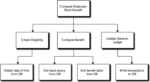
Functional decomposition was both powerful and appealing. It was powerful because it was ideally suited to managing complexity in the Turing world of an algorithmic calculating machine, especially when the 3GLs provided procedures as basic language constructs. In a world full of complex algorithms, functional decomposition was very intuitive, so the scientific community jumped on functional decomposition like tickets for a tractor pull on Hard Liquor and Handgun Night.

It was appealing because it combined notions of functional isolation (e.g., the limbs of the tree and the details of the subdivided functions), programming by contract in that the subdivided functions provided services to higher-level clients, a road map for top-down development once the decomposition tree was defined, APIs in the form of procedure signatures, very basic depth-first navigation for flow of control, and reuse by invoking the same limb from different program contexts. Overall it was a very clever way of dealing with a number of disparate issues.

Alas, by the late ’70s it was becoming clear that SD had ushered in a new set of problems that no one had anticipated. Those problems were related to two orthogonal realities:

• In the scientific arena algorithms didn’t change; typically, they either stood the test of time or were replaced in their entirety by a new, superior algorithms. But in arenas like business programming, the rules were constantly changing and products were constantly evolving. So applications needed to be modified throughout their useful lives, sometimes even during the initial development.

• Hierarchical structures are difficult to modify.⁷

The problem was that functional decomposition was inherently a depth-first paradigm since functions can’t complete until all subdivided child functions complete. This resulted in a rather rigid up-and-down hierarchical structure for flow of control that was difficult to modify when the requirements changed. Changing the flow of control often meant completely reorganizing groups of limbs.

Another problem was redundancy. The suite of atomic functions was typically quite limited, so different limbs tended to use many of the same atomic operations that other limbs needed. Quite often the same sequence of atomic leaf operations was repeated in the same order in different limbs. It was tedious to construct such redundant limbs, but it wasn’t a serious flaw until maintenance was done. If the same change needed to be made in multiple limbs, one had to duplicate the same change multiple times. Such duplication increased the opportunities for inserting errors. By the late 1970s redundant code was widely recognized as one of the major causes of poor reliability resulting from maintenance.

To cure that problem, higher-level services were defined that captured particular sequences of operations once, and they were reused by invoking them from different limbs of the tree. That cured the redundancy but created an even worse problem. In a pure functional decomposition tree there is exactly one client for every procedure, so the tree is highly directed. The difficulty with reuse across limbs was that the tree became a lattice where services had both multiple descending child functions and multiple parent clients that invoked them, as shown in Figure 1-2.

Figure 1-2. Functional decomposition tree becoming a lattice. Shaded tasks are fundamental elements of different benefits. Dashed lines indicate crossovers from one decomposition limb to another to eliminate redundancy.

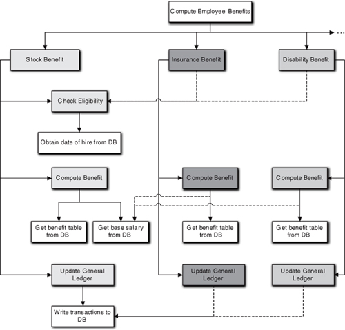
Figure 1-1 has been expanded to include the computation of multiple employee benefits that all require basically the same tasks to be done.⁸ Some tasks must be implemented in a unique way so the basic tree has the same structure for each benefit. But some tasks are exactly the same. To avoid redundancy, those nodes in the tree are reused by clients in different benefit limbs of the tree. This results in a lattice-like structure where tasks like Get base salary from DB have multiple clients that are in quite different parts of the application.

That lattice structure was a major flaw with respect to maintainability. When the requirements changed for some higher-level function (e.g., Insurance Benefit in Figure 1-2) in a particular limb, the change might need to be implemented in a descendant sub-function much lower in the tree. However, the sub-function might have multiple clients from other limbs due to reuse (e.g., Get base salary from DB). The requirements change might not apply to some of those clients that were in different limbs (e.g., Stock Benefit) because each limb where the sub-function was reused represented a different context. Then the low level change for one client might break other clients in other contexts.

The biggest difficulty for functional decomposition, though, was the implicit knowledge of context that came with depth-first processing. The fundamental paradigm was Do This. Higher-level functions were essentially just a collection of instructions to lower-level functions to do things. To issue an instruction to do something, the higher level function must (a) know who will do it, (b) know that they can do it, and (c) know that it is the next thing to do in the overall solution. All of these break functional isolation to some extent, but the last is most insidious because it requires that the calling function understand the much higher-level context of the whole problem solution. The higher-level function hard-wires that knowledge in its implementation, so when requirements changed for the overall context, that implementation had to be changed. This hierarchical functional dependence, combined with all the other problems just mentioned, resulted in the legendary spaghetti code.

Another way to look at this is through the idea of specification and DbC contracts. When a function is invoked, there is a Do This contract with the client invoking the function. That DbC contract represents an expectation of what service the function will provide. It does not matter whether the function provides the entire service itself (i.e., it is not subdivided) or delegates some or all of its functionality to lower-level functions. From the client’s perspective, the contract with the function in hand is for the entire service. If the function in hand is a higher-level function in the tree, the specification of what that function does is the specification of all of the descending limbs. The lower-level functions descending from the higher-level functions are extensions of it, and their individual specifications are subsets of the higher-level function’s specification.

This means that all of the limbs descending from a given higher-level function in the lattice form a complex dependency relationship originating with the higher-level function. That is, to fulfill its responsibilities in the DbC contract with its client, a higher-level function depends on every descendant lower-level function doing the right thing with respect to its client’s expectations. It is that dependency chain that is the real root cause of spaghetti code. A lower-level function’s specification cannot be changed without affecting a potentially long chain of parent (client) specifications.

A similar dependency problem existed for sequences of operations. To modify the sequence in which the leaf functions were invoked, the implementations of the higher-level functions had to be touched. That is, the sequence was determined by moving up and down the limbs in a systematic, depth-first manner. That navigation of the tree was hard-coded in the higher-level functions’ implementations. So to change the sequence, the implementations of multiple higher-level functions had to be changed. In effect, the overall solution flow of control was hard-wired into the tree structure itself, which sometimes required reorganizing the entire tree to accommodate small sequencing changes.

One way this is manifested is in doing unit tests of higher-level functions. Since the specification of the higher-level function includes the specification of every descending lower-level function, it is not possible to unit test a higher-level function from the client’s perspective without working implementations of every descending lower-level function.⁹

It is not terribly surprising that no one anticipated these problems. They only showed up when SD’s productivity gains were realized. As applications became larger, there were more requirements changes. Meanwhile, the functional decomposition trees were growing in size and complexity. Only when the benefits were realized did the problems show up.

Lessons Hard Won

By the time the academicians began to ruminate about OT in the late ’70s, a lot of crappy software had been written—enough so that the patterns that were common in that crappy software started to be painfully obvious. This led to a lot of papers and letters like Dijkstra’s classic, “Go To Statement Considered Harmful” in 1968.¹⁰ Those patterns represented the rather painfully learned lessons of software development (some of which were just touched on).

Global Data

One basic problem was that persistent state variables were recording the state of the system, and they were getting changed in unexpected ways or at unexpected times when they were globally accessible. This led to errors when code was written assuming a particular state prevailed and that code was later executed when that state did not prevail.

In practice such problems were difficult to diagnose because they tended to be intermittent. There was also a maintenance problem because it was difficult to find all the places where the data was written when, say, some new condition had to be added. So unrelated maintenance tended to introduce new bugs. This problem was so severe that by the late ’70s every 3GL IDE had some sort of Find/Browse facility so that you could easily search for every place a variable was accessed. While convenient for the developer, such facilities didn’t really help manage the state data properly. The problem was so pronounced that a functional programming paradigm was developed in parallel to the OO paradigm, largely to eliminate the need for persistent state data.

Elephantine Program Units

Once upon a time a fellow asked a colleague why he was getting a particular compiler error. The colleague hadn’t seen the message before, but it sounded like some compiler’s stack had overflowed, so the colleague took a glance at the code. The procedure where the error occurred was 1800 statements long, and there were several procedures of similar size in the file. Printing the compiler listing used nearly half a box of paper! Since the compiler was doing file-level optimizations, it had too much to think about and committed seppuku.

As soon as the colleague saw the length of the routine he suggested that the basic solution was Don’t Do That. At that point the code author indignantly lectured him for ten minutes on how screwed up the compiler was because it didn’t allow him to code in the most readable fashion—like nested switch statements that extend for ten pages are readable! The sad thing about this anecdote was that it occurred around 1985 when people were supposed to know better.

Huge program modules led to loss of cohesion. The modules do too many things, and those things tend to have relationships that were all too intimate within the module. That tended to make them more difficult to maintain because changes to one function are not isolated from the other functions in the module. Another common problem was mixed levels of abstraction. Such modules tended to mix both high-level functionality and low-level functionality. This obscured the high-level processing with low-level details, a classic forest-and-trees problem.

Perhaps the worst problem of all, though, was that the larger the module, the more interactions it tended to have with other modules, so the opportunities for side effects were greatly increased. All modern approaches to more maintainable code advocate limiting the scope where side effects can occur. The simplest way to limit scope is to keep modules small.¹¹

Software Structure

The word architecture started to appear in the software literature in the ’70s because people were coming to understand that a software application has a skeleton just like a building or an aardvark. The painful lesson about structure is that when it has to be changed, it usually requires a great deal of work. That’s because so much other stuff in the application hangs off that structure.

There are four common symptoms that indicate structural changes are being made to an application:

1. Lots of small changes are made.
2. The changes are spread across many of the program units.
3. Changes are difficult to do (e.g., hierarchies have to be redesigned).
4. The changes themselves tend to introduce more errors and rework than normal.

Such changes are commonly called Shotgun Refactoring, and in the Hacker Era there was a whole lot of it.

Lack of Cohesion

One correlation that became apparent early on was that changes were being made to many modules when the requirements changed. One reason was that fundamental structure was being modified. The other was lack of cohesion. Functionality was spread across multiple modules, so when the requirements for that functionality changed, all the modules had to be touched. Lack of cohesion makes it difficult to figure out how to modify a program because the relevant functionality is not localized. Because different modules implemented different parts of a given functionality, those implementations tended to depend on one another to do certain things in particular orders. Although it was usually easy to recognize poor cohesion after the fact, there were no systematic practices that would guarantee good cohesion when the application was originally developed.

Coupling

There have been entire books written about coupling and how to deal with it, so the subject is beyond the practical scope of this book. At the executive summary level, coupling describes the frequency, nature, and direction of intimacy between program elements. The notion of logical coupling grew out of trying to reconcile several different observations:

• Spaghetti code is difficult to maintain.

• Bleeding cohesion across modules resulted in implementation dependencies between them.

• If a client knows a service intimately, it often has to change when the service changes.

• If a service knows a client intimately, it often has to change when the client changes.

• The need to change two elements at once is directly proportional to the nature of access between them.

• The need to change two elements at once is directly proportional to the intimacy of access between them.

• Bidirectional intimacy is usually worse than unidirectional intimacy.

So the notion of coupling arose to describe dependencies between modules resulting from interactions or collaborations between program units. Alas, for a program to work properly, its elements must interact in some fashion. Consequently, developers were faced with a variation on the Three Laws of Thermodynamics: (1) You can’t win; (2) You can’t even break even; and (3) You can’t quit playing.

When thinking about coupling it is important to distinguish between logical and physical coupling. Logical coupling describes how program elements are related to one another based on the roles they play within the problem solution. Physical coupling describes what they need to know about each other to interact from a compiler’s perspective. Logical coupling in some fashion is unavoidable because solving the problem depends upon it. But it can be minimized with good design practice.

Physical coupling, though, is almost entirely due to the practical issues of implementing 3GL-type systems within the constraints of hardware computational models. For the compiler to write correct machine code in one module for processing—say, data passed to it from another module via a procedure call—the compiler must know how that data was implemented by the caller (e.g., integer versus floating point). Otherwise, the compiler cannot use the right ALU instructions to process it. So the compiler needs to know about the implementation of the calling module, which is a physical dependency on that implementation that is dictated by the particular hardware. The most obvious manifestation of this sort of coupling is compile-the-world, where many modules in a large application must be recompiled even though only one had a simple change.

Unfortunately, the literature has been concerned primarily about the frequency of access. Only in the late ’80s did the deep thinkers start worrying about the direction of coupling. They noticed that when the graph of module dependencies was a directed graph without loops, the program tended to be much more maintainable. They also noticed that very large applications were becoming infeasible to maintain because compile times and configuration management were becoming major headaches. The challenge lies in minimizing or controlling the physical dependencies among program elements. The techniques for doing this are generally known as dependency management.

To date the literature has rarely addressed the nature of coupling. Since the nature of coupling plays a major role in justifying some MDB practices, it is worth identifying here a basic way of classifying the nature of coupling (i.e., the degree of intimacy), in order of increasing intimacy:

• Message identifier alone. This is a pure message with no data and no behavior. The opportunities for foot shooting are quite limited, but even this pristine form can cause problems if the message goes to the wrong place or is presented at the wrong time.

• Data by value. This form is still pretty benign because there is no way to distress the sender of the message and the receiver has full control over what is done with the data. It is somewhat worse than a pure message because the data may no longer be correct in the program context when the message is processed. This is usually only a problem in asynchronous or distributed environments when delays are possible between sending and processing the message. It can also be a problem in threaded applications where parallel processing is possible.

• Data by reference. Here we have the added problem of the receiver being able to modify data in the sender’s implementation without the sender’s knowledge. Data integrity now becomes a major issue. In fact, passing data by reference compounds the problems in the parallel processing environments because the receiver (or anyone to whom the sender also passed the data by reference) can change it while the sender is using it.

• Behavior by value. This curious situation arises in modern programs that pass applets in messages. This is similar to data-by-reference except that it is the receiver who can be affected in unexpected ways. The reason is that the applet is in no way constrained in the things that it does. When the receiver invokes the behavior it effectively has no control over and cannot predict a potentially unlimited number of side effects. If you don’t think applets are a problem, ask anyone who deals with web site security.

• Behavior by reference. Though some languages from previous eras could do this by passing pointers to functions, it was very rare. Alas, in OOPLs it can be done trivially by passing object references. Like FORTRAN’s assigned GOTO, it probably seemed like a good idea at the time, but it turned out badly. Today we realize this is absolutely the worst form of coupling, and it opens a huge Pandora’s Box of problems. In addition to invoking behavior with potential for all sorts of side effects, the receiver can also change the object’s knowledge without the sender knowing. Since the class’ entire public interface is exposed, the receiver is free to invoke any aspect of the object, even those aspects that would cause a problem for the sender.

But worst of all, the encapsulation of the sender has been totally trashed. The reason is that the object whose reference is passed is part of the sender’s implementation.¹² By passing it, a bay window has been opened into the implementation of the sender that invites bugs and presents a maintenance nightmare. (In OO terms, it defeats implementation hiding, which is a fundamental OO practice.) This means the maintainer must track down every place the reference is used and verify that any change to the way it is used won’t break anything. Even then, we can’t be sure that someone won’t change the receiver during another bout of maintenance to access the instance incorrectly. And even if everything just works, one still has to rebuild the receiver because of the physical coupling.

Because it is such a broad topic, space precludes dealing with coupling in this book. But it is important to note that the notion of coupling formalizes a flock of maintainability issues, and understanding coupling is fundamental to good program development whether you are doing OO development or not.

Technical Innovation

Prior to the OO paradigm all was not chaos, even in the Dark Ages of programming. The academicians were busily adapting mathematics to practical use in the computing environment. During their cogitations the academicians provided a mathematical lingua franca for the underpinnings of software development. This was a collection of theories and models that were particularly well suited to the computing environment. Today this mathematics is the basis of almost everything we do in software development.

This book takes an engineering approach to software development, so it is not going to trot out a lot of theorems. It is, however, worth a couple of subsections to briefly describe at the megathinker level the major relevant mathematical elements and how they influence software development. That’s because those ideas still underlie the OO paradigm, albeit in a very well-disguised manner.

The Turing Machine

In the 1930s Alan Turing developed a detailed mathematical model of a theoretical calculating machine. The model was elegantly simple. It assumed all calculating processes were divided into fundamental, individual steps. Those steps could be expressed as a small set of atomic instructions to his machine. Once so divided any calculating process could be described in the following terms:

Sequence: A sequence of one or more instructions located consecutively in the program

Branch: A shift in the execution of the program from a sequence in one program location to another sequence at a different location in the program based upon the truth of some boolean condition

Iteration: A combination of sequence and branch that allowed a sequence to be repeated indefinitely until some boolean condition became true

The mathematics became heavily involved with precise definitions of things like instruction and condition, and then proving that a Turing machine with a finite instruction set could, indeed, successfully perform any arbitrarily complex calculation. To do so Turing had to examine various strategies for combining and nesting the basic operations.

The Turing machine is the most famous, but there have been a succession of models of computation developed over the years. These models belong to the general class of hardware computational models. It is important to realize that such models describe how a computer works, not how software is designed. In reality, almost the entire computing space is based upon various hardware computational models. Even exotic mathematical constructs like 3GL type systems have their roots in hardware computational models.

The OO paradigm represents the first major break away from the hardware computational models in creating an approach to software design that is, at least in part, independent of the hardware computational models.¹³ That is not to say, though, that the OO paradigm ignores those models. Ultimately the problem solution has to be executed on Turing hardware, so the OO paradigm necessarily has to provide an unambiguous mapping into the hardware computational models.

Languages and Methodologies

As suggested, programs are written in a variety of languages. Initially programs were encoded as binary instructions directly into the hardware on plug boards that directly connected power rails to the hardware to form logic 1 and logic 0, one bit at a time. Instructions to the Arithmetic Logic Unit (ALU) consisted of binary words of a fixed size written directly into hardware registers. This was complicated by the fact that the hardware commonly subdivided those words into bit subsets called fields.

The first major advance in software development was the introduction of BAL.¹⁴ As bigger problems were solved, software programs became larger, but people don’t think well in binary. BAL enabled hardware operations to be described symbolically with mnemonics like ADD, MOV, and JMP. BAL also enabled ALU registers to be represented symbolically as R1, R2, . . ., Rn. Finally, BAL enabled the developer to assign mnemonic names to memory addresses so that data could be named in a meaningful way. All these things were a boon to software development because they allowed the developer to think about the solution in more abstract terms than endless strings of 1s and 0s.

However, for BAL to work, all those mnemonics had to be translated into the binary view that the hardware understood. Thus was introduced the powerful notion of a program, called a compiler, to process other programs by converting them from one representation to another. (Primitive operating systems were already around to manage the housekeeping around running programs through the ALU, but they didn’t significantly modify those programs.)

While all this made life much, much easier for the early software developers, there were still some problems. BAL was necessarily tied to the specific ALU instruction set, and by the 1950s hardware vendors were churning out a wide variety of computers with different instruction sets. What was needed was a more abstract description of the solution that was independent of a particular instruction set. This led to the introduction of FORTRAN (FORmula TRANslator) and COBOL (COmmon Business-Oriented Language) in the late 1950s. Just as BAL raised the level of abstraction of software programs above binary expression, this next generation of languages raised the level of abstraction above the ALU itself.

These 3GLs introduced a number of new abstract concepts for computing. These are the primary ones that characterized that generation of languages.

• Procedures. Procedures were blocks of instructions that could be invoked from anywhere in the program. When the block completed, control would return to the point in the program from which the procedure was invoked. This enabled a suite of instructions to be reused in different contexts, which was quite common in large applications.

• Procedural message passing. However, the data that was modified for each invocation context of a procedure needed to be different. Procedure parameters enabled a particular context to provide data that was unique to that context. Then such parametric data became a unique message sent to the procedure by an individual invocation context. This went a long way toward decoupling what the procedure did with the data from the source context of the data.

• Types. To provide that decoupling an abstract mechanism was needed for describing generally what the data is without the detailed semantics of source context. Types allowed the data to be defined for the procedure very generically (e.g., as an integer value). Thus a procedure to compute statistics on a bunch of samples could do so without knowing what the samples actually were; it only needed to know they were integers to compute things like means and T-Statistics. Thus, types at the 3GL level initially defined the implementation of data rather than the problem semantics of the data.

• Stack-based scope. Since procedures were called from other procedures, there was an inherent hierarchical structure for sequences of operations. Procedures needed to know how to get back to where they came from, and the notion of a call stack was born. The call stack provided a way to keep track of where you came from so that you could unravel nested procedure calls as they completed their tasks.

• Procedural block structuring. Procedures provided very useful building blocks for isolating functionality. Such modularity enabled a divide-and-conquer approach to managing complexity. The 3GLs extended this idea to provide modularity within procedures. This supported hard-won lessons like programs being more robust when groups of instructions had single entry and exit points.

Thus the 1960s was a time of profound revolution as software development moved from BAL to 3GLs. New concepts like procedural message passing and stack-based scope required a different view of construction than the only slightly abstracted Turing view of computing in BAL. Into the breach stepped the methodologists. As soon as 3GLs became widely accepted, the need for training developers in using them properly arose.¹⁵ By the early 1970s it was clear that the larger programs enabled by 3GLs needed to be properly designed. That gave birth to a host of construction approaches under the general umbrella of Structured Development, as discussed previously.

Basically, those approaches recognized that solving large problems requires something more that just Assembly or 3GL coding skills. Somehow all those abstract constructs needed to play together properly to solve the customer’s overall problem. Not the least of the problems was the recognition that programs needed to be maintainable. In addition, large programs needed a structural skeleton and, once in place, that skeleton tended to be very difficult to modify because of the sheer number of disparate constructs hanging off it. So the methodologies quickly evolved to a more abstract level than 3GL coding, and the developer started looking at the Big Picture as a separate design activity from 3GL coding.

Programming languages are not the only representations of executables. There have been a large number of pictorial notations used to describe programs. It is no accident that every design notation from early HIPO charts¹⁶ to today’s Universal Modeling Language (UML) are often referred to as graphical notations. Such notations can express the abstract concepts needed for design very efficiently.

Most of the readers of this book will have some software development experience, so the previous discussion of languages and methodologies will probably be quite familiar. However, it was worth the review because there are several important things the rest of the book builds upon.

• A problem solution expressed in any language above binary machine language is a more abstract representation of the machine language that will actually execute on the Turing Machine. Another word for abstract representations of something more concrete is model. Thus a program in C is a model of the problem solution that will ultimately execute on the computer in the same sense as a UML OOA model is.

• Software development is continuously evolving towards more abstract ways of expressing problem solutions.

• Because of the ubiquitous presence of mathematics in the computing environment, the computing space is deterministic. For example, compilers, linkers, and loaders automated a lot of drudge work for early BAL and 3GL developers because mapping things like symbolic names to binary addresses is deterministic, even for complex multitasking environments.

Sets and Graphs

It is beyond the scope of this book to describe how ubiquitous various mathematics, especially set and graph theory, are in the computing space. However, a few implications of that are very important to the OO paradigm and MBD in particular.

• The computing space is deterministic. That’s because some kind of rigorous mathematics underlies everything in it, however well disguised that might be. This has enormous implications for automation.

• The computing space is disciplined. Everywhere we turn we are constrained by rules like those for language syntax, data structures, identity, GUI design, and so forth. In reality there is very little freedom in implementing problem solutions once we have defined the specific computing environment. Creativity in software development lies in designing solutions, not implementing them.

• The computing space is ultimately based on hardware computational models. However abstract our solution constructs are, the underlying mathematics ensures that they will all map unambiguously into hardware computation.

• The first methodological step in any software construction is expressing the ill-defined, imprecise, ambiguous notions of non-Turing customer spaces in notations that are complete, precise, and unambiguous with respect to the computing space. The mathematics underlying those notations that enable rigorous expression must necessarily be the same mathematics that underlies the computing space.

The methodologies of SD were not simply encyclopedias of a potpourri of hard-won lessons learned in the development trenches prior to 1970. Instead, they became cohesive philosophies of software construction that were based on solid mathematics. Every software construction methodology that has stood the test of time sits on that sort of mathematical platform, however informal its exposition might be and however simple its notation might seem. This was a two-way street; computing has been the driving force in developing entirely new branches of mathematics, from relational theory through type theory to exotic topological theories for non-Turing computation.

Normal Form (NF)

One of the most useful tools to evolve concurrently with SD was a particular branch of general set theory that underlies data storage and the static description of programs. That is, it formalizes and constrains the way data is defined, modified, and related to other data. E. F. Codd first defined it in the late ’60s to describe relational databases.¹⁷

Codd’s Relational Data Model (RDM) has since been incorporated into both the OO paradigm and extensions of SD. For example, the descriptor attribute associated with knowledge in OO classes is a term Codd introduced in 1970. A suitably arcane branch of mathematics with much broader scope has since been developed, called relational theory. The OO paradigm is based on that broader view.

We can avoid the mathematics of the set theory that forms the basis of NF here and provide the executive summary view because all one needs to know to develop good applications are the implications of the theory. Though NF is more broadly applied, it is most easily understood in terms of tables. The table itself represents an n-ary relation of table entities (the rows) that each share the same n attributes (the columns). That is, the table describes a set of entities that share characterization in terms of the attributes. Each attribute identifies a particular semantic domain of possible values. Each table entity (a row or tuple) has a unique identity and a set of specific values (the table cell values) for the attributes (see Figure 1-3).

Figure 1-3. Mapping of problem space entities to an n-ary relation. Each identifiable entity becomes a tuple in the relation. Each relation captures a set of unique values of characteristics that are common to each entity.

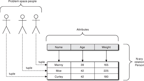
In more practical terms, a column attribute represents a particular data semantic that is shared by every row in the table; it describes what the data in the cells of that column is. The cells then represent specific values for that semantic. Then each row represents a set of attribute values that is uniquely associated with the entity. The uniqueness is tied to identity; each row must have a unique identity that distinguishes it from other rows, and the attribute values must depend on that identity. In Figure 1-3 that identity is the name of a person.

In the more restrictive relational data model that applies to databases, some subset of one or more embedded attributes comprises a unique identifier for the table row, and no other row may have exactly the same values for all the identifier attributes. The identifier attributes are commonly known collectively as a key. Other attributes that are not part of the key may have duplicated values across the rows, either singly or in combination. But the specific values in a given row depend explicitly on the row key and only on the row key.

Relational theory is about the ways particular entities in different n-ary relations (tables) can be related to each other. For that theory to be practically useful, there need to be certain rules about how attributes and entities can be defined within an nary relation. That collection of rules is called normal form, and it is critical to almost all modern software development.

The kernel of NF has three rules for compliance:

1. Attributes must be members of simple domains. What this essentially means is that attributes cannot be subdivided further (i.e., their values are scalars). That is, if we have a table House with attributes {Builder, Model}, we cannot also subdivide Model into {Style, Price}. The problem is that the Style/Price combinations would be ambiguous in a single-valued attribute cell for Model in a row of House. So the House table must be composed of {Builder, Style, Price} instead.
2. All non-key attributes, compliant with 1st NF, are fully dependent on the key. Suppose a House table is defined with attributes {Subdivision, Lot, Builder, Model} where Subdivision and Lot are the key that uniquely identifies a particular House. Also suppose only one builder works on a subdivision. Now Builder is really only dependent upon Subdivision and is only indirectly dependent upon Lot through Subdivision. To be compliant we really need two n-ary relations or tables: House {Subdivision, Lot, Model} and Contractor {Subdivision, Builder}. (The RDM then provides a formalism that links the two tables through the Subdivision attribute that can be implemented to ensure that we can unambiguously determine both the Model and the Builder values for any House. That notion is the subject of a later chapter.)
3. No non-key attributes, compliant with 2nd NF, are transitively dependent upon another key. Basically, this means that none of the non-key attribute values depend upon any other key. That is, for House {Subdivision, Lot, Model}, if we have a Subdivision = 8, Lot = 4, and Model = flimsy, the Model will remain “flimsy” for Subdivision = 8 and Lot = 4 regardless of what other rows we add or delete from the table.

Generally, most developers depend on the following mnemonic mantra to deal with 3rd NF: An attribute value depends on the key, the whole key, and nothing but the key.

Other NF rules have been added over the years to deal with specialized problems, especially in the area of OO databases. We won’t go into them here because they are not terribly relevant to the way we will build application models and produce code. However, the value of the three normal forms above is very general and is particularly of interest when defining abstractions and their relationships.

Data Flows

Data was a second-class citizen until the late 1960s.¹⁸ Most of the early theoretical work in computer science was done in universities where the computer systems were solving the highly algorithmic problems of science and engineering. However, by the late 1960s there was an epiphany when people became aware that most of the software in the world was actually solving business problems, primarily in mundane accounting systems.

In particular, business problems were not characterized by algorithms but by USER/CRUD¹⁹ processing of data.²⁰ For one thing, core business problems were not algorithmic rocket science—doing a long division for an allocation was pretty cutting edge.²¹ On the other hand, those very simple calculations were done repeatedly on vast piles of data. What the business community needed was a way to handle data the same way the scientific community handled operations. This led to various flavors of data flow analysis. The basic idea was that processes were small, atomic activities that transformed data, and the processes were connected together by flows of data, as illustrated in Figure 1-4.

Figure 1-4. Example of data flow diagram for computing whether a retirement gift should be given to an employee. Data is provided as flows (e.g., Employee ID and age) or is acquired from data stores (e.g., Date of birth and Today’s date).

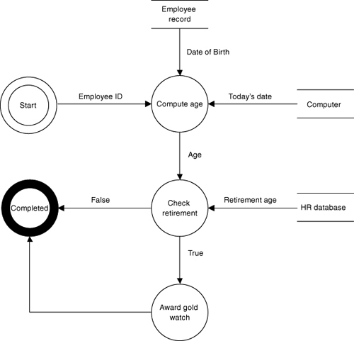
As it happens, when we make a data flow graph, it represents a breadth-first flow of control. The processes are self-contained and atomic rather than decomposed. So the problem solution is defined by the direct connections between those processes. The connections are direct and depend only on what needs to be done to the data next. If we want to solve a different problem, we change the connections and move the data through the same atomic processes differently. Data flows represented a precursor of the peer-to-peer collaboration that is central to the OO paradigm and will be discussed in detail later.

Alas, this view of the world did not mesh well with the depth-first, algorithm-centric view of functional decomposition. Trying to unify these views in a single software design paradigm led to some rather amusing false starts in the ’70s. Eventually people gave up trying and lived with a fundamental dichotomy in approaches. For data-rich environments with volatile requirements, they focused on the OO paradigm as the dominant paradigm. Meanwhile, functional programming evolved to deal with the pure algorithmic processing where persistent state data was not needed and requirements were stable.

In many respects the purest forms of data flow analysis were the harbingers of the modern OO paradigm. As we shall see later, the idea of small, self-contained, cohesive processes has been largely canonized in the idea of object behavior responsibilities. Ideas like encapsulation and peer-to-peer collaboration have driven a breadth-first flow-of-control paradigm. But in two crucial respects they are quite different. The OO paradigm encapsulates both the behavior and the data in the same object container, and the data flows have been replaced with message flows. The important point to take away from this subtopic is that where SD was based on functional decomposition, the OO paradigm is more closely aligned with data flows.

State Machines

Meanwhile, there was another branch of software development that was in even deeper trouble than the business people. Those doing real-time and/or embedded (R-T/E) hardware control systems were experiencing a different sort of problem than maintainability. They just couldn’t get their stuff to work.

Basically they had three problems. First, such control systems were often used in environments that were extremely resource limited. They didn’t have the luxury of stuffing an IBM 360 into a washing machine or railroad signal. Second, the supporting tools that other developers used weren’t available in their environment. This was especially true for debugging programs when they might not even have an I/O port for print statements, much less a source-level debugger.

The third problem was that they were dealing with a different view of time. Events didn’t happen in synchronization with predefined program flow of control; they occurred randomly in synchronization with the external hardware, and that external hardware never heard of Turing unless it happened to be a computer. Their asynchronous processing completely trashed Turing’s ordered world of preordained sequence, branch, and iteration. The tools have gotten better over the years, but the R-T/E people still have the toughest job in the software industry.

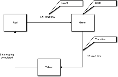
The tool that made life bearable for the R-T/E people was the Finite State Machine (FSM).²² We have no idea who first wrote a program using an FSM, but whoever it was deserves to be in the Software Hall of Fame along with Ada Lovelace and crew. It basically enabled asynchronous processing in a serial Turing world. It also made marvelously compact programs possible because much of the flow of control logic was implicit in the FSM rules for processing events and static sequencing constraints represented by transitions, as shown in Figure 1-5.

Figure 1-5. Example of a finite state machine for a simple traffic light. The traffic light migrates through states in a manner that is constrained by allowed transitions. Transitions from one state to the next are triggered by external events.

However, the really interesting thing about FSMs is that they happen to address a number of the same issues that are the focus of OOA/D. In particular, they provide an extraordinary capability for reducing the degree of coupling and truly encapsulate functionality. They also enforce basic good practices of OO design. If we were given the task of coming up with a single construct to capture and enforce core elements of the OO paradigm, the FSM would be that construct. But we will defer the discussion of how that is so until Part III.