

10.1 Introduction
For the most part, conventionally designed directional antennas have considered operation only at the carrier frequency with little regard for bandwidth. More recently, however, the new modulation schemes raise questions concerning the actual bandwidth of a conventionally designed AM directional antenna, so it is useful to have a capability that provides some insight into that subject.
This chapter extends the application of NEC-2 to include the total system—antenna-matching networks, phasing networks, and other parts of the system including the transmission lines. The resulting analysis views the bandwidth of the total system plus the bandwidth at some intermediate points along the signal path.
The material in this chapter draws heavily from a paper the author submitted to IEEE Transactions on Broadcasting, in which the calculations were performed using NEC-4 rather than NEC-2. Although this difference might cause a minor variation in the numerical values displayed in the charts, the methods and procedures are identical in both codes and the conclusions reached will be the same.
10.2 System Definition
By definition, the antenna system consists of all networks and transmission lines beginning at the common point fed by the transmitter and continuing through the tower radiators. As you progress through this chapter, it will immediately be obvious that the system performance of a conventionally designed directional antenna system is well behaved at the carrier frequency: Everything that is supposed to be 50 Ω is, in fact, 50 Ω. Everything that is supposed to be j0 is indeed j0. But when viewed over the signal bandwidth, the system performance might vary surprisingly from the ideal.
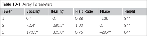
In an attempt to seek a balance between being overly simple and excessively complicated, a three-tower array will be used as the vehicle to illustrate the concepts involved when analyzing the total system. The hypothetical system operates on a frequency of 850 kHz with a power of 5000 watts. The array parameters are given in Table 10-1.
The transmission line lengths are 725 feet, 468 feet, and 906 feet for towers 1, 2, and 3, respectively. Figure 10-1 is a simplified block diagram of the system.
10.2.1 Tower Models
This chapter provides another demonstration of modeling towers using the lattice tower model described in Chapter 3.
In creating the lattice tower model, the concrete tower base with four ground straps and the base insulator complete with spider and girth (as shown in Figure 10-2) are modeled using normal NEC-2 procedures.
Then a single tower section consisting of three upright legs with a three-wire top girth is modeled and repeated twenty-six times to stack twenty-seven 10-foot sections on end to complete the first tower.
Once the first tower is completely modeled, it is duplicated to generate the other two towers by using the GM command to translate the entire assembly to the proper locations. The details of how this is done are not repeated here since they have been covered previously.
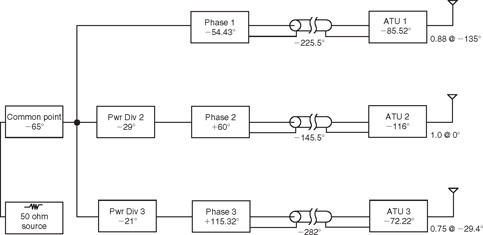
FIGURE 10-1![]()
System block diagram.
FIGURE 10-2![]()
NVCOMP.EXE view of lattice tower model.
There is, however, one item of interest in this tower geometry worth mentioning here. The wire simulating the base insulator and upon which the excitation is placed is 0.6731 meters long. Since it is desirable to have equal-length segments on both sides of the feed segment, a means to accomplish that goal is demonstrated on the tower section immediately above the insulator by dividing the section into three segments instead of the usual one, and then using the GC continuation command to taper the length of those three segments starting with 0.6731 meters (to equal that of the feed segment), and increasing with the ratio 1.4438:1 to approach 3.048 meters, which is the length of the tower sections above it. The following commands implement that segment taper on the three tower legs.
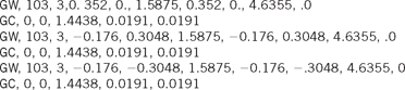
The GW wire specification in Appendix A contains information on using the GC continuation command, including a formula to calculate the segment ratio that will yield the desired starting segment length. It is a good idea to read that material at this time.
10.2.2 Tower Base Drive Voltages
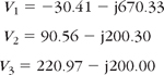
The normalized base drive voltages necessary to create the desired pattern were calculated using the procedures described in Chapter 6 with the following results:
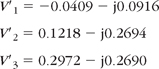
The normalized base drive voltages were then scaled to obtain the full power drive of
These drives were placed in the NEC-2 input file and run to obtain the output file. This is where the effort would have normally ceased but in this instance, we will continue to include a study of the total system.
10.3 Bandwidth Analysis
The array characteristics as a function of frequency are easily obtained by making NEC-2 runs at the several frequencies of interest, in this case 850 kHz ± 20 kHz with intervals of 5 kHz. While a method is provided in the FR command for stepping the frequency through such a range, that method cannot be used for this analysis because the directional antenna system uses matching and phasing networks that are described in NEC-2 using NT commands. Each network is defined in the NT command by its frequency-sensitive Y-parameters and, unfortunately, NEC-2 does not scale the Y-parameters with frequency. Thus it will be necessary to specify a fixed frequency with the associated network commands written to that frequency, generate the required data, then change both the frequency and the network commands to a second frequency, generate that data, and so on.
In addition, it is important to note that NEC-2 requires that all network commands be grouped together so when one NT command is changed, all the unchanged network commands must be repeated to create a new and complete group. Moreover, be aware that NEC-2 considers transmission lines to be a special case of the network. Therefore, notwithstanding the fact that the TL commands are indeed scaled with frequency, they must nevertheless be included and repeated in each new group along with the NT commands.
10.3.1 Source Impedance of the Drive Voltage
The voltage source provided in NEC-2 by the EX command is a constant voltage with zero source impedance. During a normal NEC-2 design at the carrier frequency, where all networks and tower currents are designed and adjusted for the carrier frequency, source impedance of the drive voltage is not necessarily a factor. In practice over a bandwidth, however, when the load being driven by the voltage source varies with frequency, it causes the applied voltage to be a function of frequency depending on both the source impedance of the drive and the varying load impedance. This is especially noticeable when using NEC-2 to determine the various tower drive point impedances of an array over a bandwidth.
When driving a network or transmission line having a 50-ohm input, a 50-ohm voltage source can be created in NEC-2 by driving through a network containing a single 50-ohm series resistor, such as the one shown in Figure 5-2(b). However, a special frequency-sensitive impedance source replicating that of the output impedance of the antenna-tuning unit (ATU) is required to measure the bandwidth of the drive point impedance of an operating array's towers. This is necessary because the drive point impedance of the operating tower is a function of the drive voltage, which in itself is a function of the frequency-sensitive source impedance. This rather circular requirement can be met by driving each tower through its ATU with a 50-ohm-voltage source feeding the ATU. This yields both the frequency behavior of the ATU input impedance as read from the NEC-2 output file under the heading - ANTENNA INPUT PARAMETERS - as well as the tower drive point impedance, which is read from the same report under the heading - STRUCTURE EXCITATION DATA AT NETWORK CONNECTION POINTS -.
Figure 10-3(a) displays the effect that the source impedance can have in calculating the tower drive point resistance when driving the towers through their respective ATU. The figure shows tower 2 drive point resistance when the ATU is driven first with a drive source impedance of 0 ohms and then again when the ATU is driven using a drive source impedance of 50 ohms. Figure 10-3(b) shows the resistance seen looking into ATU 2 input when driving the ATU with a voltage of 0 source impedance, then driving it with a voltage having 50-ohm source impedance.
These curves were taken by simultaneously driving the inputs of the three ATUs with the voltages necessary to generate the desired field ratios at the carrier frequency and then varying the frequency as shown. The ATUs were driven first with the normal 0 source impedance of the NEC-2 EX command, then again with a 50-ohm source obtained with the EX command feeding the ATU through a 50-ohm network. The tower drive point impedance and the ATU input impedance were read from the NEC-2 output file.
In the interest of simplicity, only the results pertaining to the resistive part of tower 2 impedance are given in the illustrations of Figure 10-3(a) and 10-3(b). Figure 10-3(a) shows, the two sources give the same results at the carrier frequency of 850 kHz but as the frequency varies across the bandwidth, the results differ noticeably. Figure 10-3(a) also shows that driving the ATU with the zero source impedance causes the resistive part of the tower 2 impedance to go to 0 near 838 kHz. However, driving the ATU with the 50-ohm source impedance causes the resistive part of the tower 2 impedance to stay positive throughout the bandwidth.
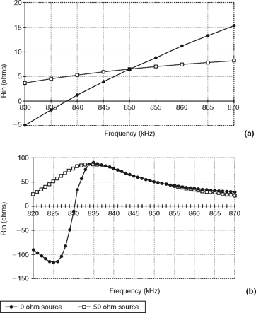
FIGURE 10-3![]()
Effect of drive source impedance: (a) tower 2 drive point resistance, (b) antenna-tuning unit 2 input resistance.
Figure 10-3(b) shows the effect this has on the input impedance of the ATU. In this instance, the drive with 0 source impedance causes the ATU input resistance to go to 0 near 830 kHz while the drive with 50-ohm source impedance causes the ATU input resistance to remain positive throughout the bandwidth. Again, notice that both drive sources give the desired 50-ohm ATU input resistance at the 850 kHz carrier frequency.
10.3.2 Intermediate Data
The figures that follow display the NEC-2 calculated impedance data as it appears at the several network interfaces shown in Figure 10-1. The data were taken using a drive with a 50-ohm source impedance.
Procedure for Calculating Intermediate Data
To calculate the data that follows, the tower drive voltages necessary to create the desired field ratios were first calculated as described in Chapter 6. A NEC-2 run was made at the carrier frequency and the tower drive point impedances were thus determined. From that information, the complete system was designed as it appeared at the carrier frequency, including ATUs, phasing networks, power dividers, and so on.
Then, the drive voltages were translated back from the tower base to the input of the ATU to obtain the ATU input drive voltages that would create the desired field ratios. A NEC-2 run was made with the drive at the input to the ATU and the field ratios generated by the translated drive voltages were calculated and verified as being the target values. The ATU input impedances and the tower drive point impedances were then read from the NEC-2 output files thus created.
While holding the network component values constant but scaling reactance with frequency, additional NEC-2 runs were made with the frequency varied ±20 kHz in 5-kHz steps to generate the bandwidth performance as viewed at the tower bases and at the ATU inputs.
Following similar procedures, the ATU drive voltages were then translated back through the transmission lines to obtain the desired drive voltages at the transmission line inputs. There additional NEC-2 runs were made as before to obtain the transmission line input impedances versus frequency.
In turn, the voltages were translated back through each of the system's functional elements until the input to the common point-matching network was reached. At each voltage translation, the field ratios thus generated were calculated to confirm that the translated drive voltages did indeed produce the target field ratios.
In translating the voltages from network to network, it is important to remember that the network phase shifts refer to current phase shift. Therefore, the current is shifted backward to the input of the network, then that shifted current is used to calculate the voltage that must appear at the network input to create that current.
Tower Base Impedances
Figures 10-4(a) and (b) show the drive point impedance of the three towers when they are driven by their respective ATUs. Little comment is needed here except to notice that the procedure described earlier was followed with the result that tower 2 shows a rather low resistance (slightly more than 6 ohms) at the carrier frequency.
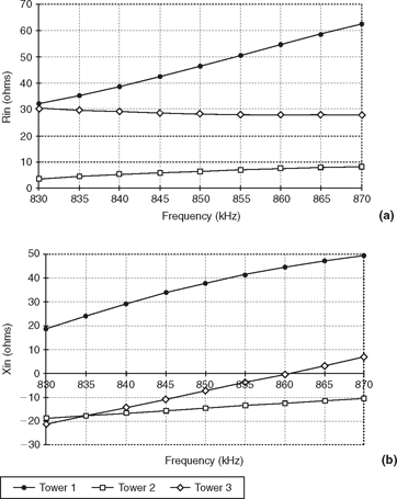
FIGURE 10-4![]()
Tower drive point impedance when driven by ATU: (a) resistance, (b) reactance.
ATU Input Impedances
Figures 10-5(a) and 10-5(b) show the input impedance to the three ATUs when they are driven with a 50-ohm source. Notice that all three ATUs show a 50 + j0 input impedance at the carrier frequency but ATU 2 varies signifiantly over the bandwidth.
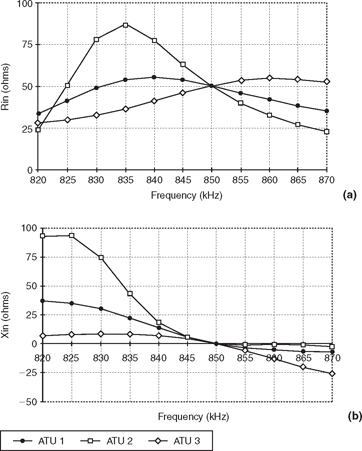
FIGURE 10-5ATU input impedance: (a) resistance, (b) reactance.
Transmission Line Input Impedances
The curves showing the input impedance of the three transmission lines are given in Figures 10-6(a) and (b). In addition, Figure 10-6(c) has been included to show the voltage standing wave ratio (VSWR) of the transmission lines.
Figure 10-6(c) shows that the ratio for transmission lines 1 and 3 remain below 2:1 throughout the bandwidth but transmission line 2 exceeds 2:1 at the extremes and is up to 3.6:1 at the low-frequency end of the bandwidth. This is an item to be concerned with when selecting the type of transmission lines, although the need for this concern is not apparent when the design is limited to the carrier frequency. In this hypothetical system, tower 2 is the low-power tower so when the transmission line is selected to accommodate the highest power, it will also accommodate the power of tower 2 even with this higher VSWR. The inverse may be true in some instances, however.
Notice, too, in Figure 10-6(a) that the fairly low input impedance of ATU 1 has been transformed to approximately 90 ohms by transmission line 1. Also note in Figure 10-6(c) that although the terminating impedance of transmission line 1 has been transformed noticeably, the VSWR on transmission line 1 is reasonable; it does not exceed 1.8:1. This is a reminder that the VSWR is the same at all positions along a transmission line but that the impedance does, in fact, vary with position along the line.
Phasing Network Input Impedances
Figures 10-7(a) and (b) show the variation in the input impedance of the phasing networks and no comment is needed.
Power Divider Input Impedances
In designing the voltage buss for the power dividers, it was elected to set the buss voltage at the voltage required to accommodate the 50-ohm impedance of the highest-power tower. With that voltage established, the input resistance of the power-dividing networks for the other two towers was defined. With all three paths paralleled, the resulting impedance was near 29 + j0 at the carrier frequency. Figure 10-8 shows how this impedance varies over the bandwidth.
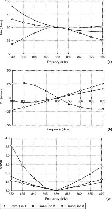
FIGURE 10-6![]()
Transmission line input impedance: (a) resistance, (b) reactance, (c) VSWR.
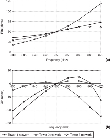
FIGURE 10-7![]()
Phasing network input impedance: (a) resistance, (b) reactance.
Notice the smoothing effect that has occurred in paralleling the three paths. The rogue tower 2 has been somewhat subdued by its better-behaved companion towers.
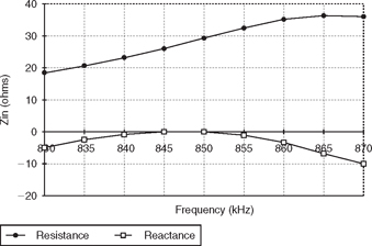
FIGURE 10-8![]()
Power divider impedance.
10.3.3 Total System Bandwidth Data
A single voltage drive of arbitrary phase at the input to the common point-matching network drives the complete system. In this analysis, the drive is through a 50-ohm network to create a 50-ohm source impedance.
The Common Point Network
The common point-matching network transforms the 29-ohm parallel combination of the three tower paths to the conventional 50 ohms. The resulting input impedance behavior of this network is shown in Figure 10-9(a) and shows the design value of 50 + j0 impedance at the carrier frequency. Unfortunately the common-point impedance fails to display the symmetry desired for digital transmissions so a phase-rotating network would be in order for that application.
Notwithstanding the antics of tower 2, the VSWR at the input to the common point-matching network remains reasonably symmetrical and below 1.5:1 over a ±15 kHz bandwidth, as shown in Figure 10-9(b).
Radiation Bandwidth
In the end, the question might be “How well does the system radiate over the bandwidth?” Some insight into that aspect of the analysis can be obtained by including an RP command in each frequency step. The parameters of this RP command are set to call for only one field calculation per frequency and for that calculation to occur at azimuth 59°, which is the peak of the main lobe of the radiation pattern.
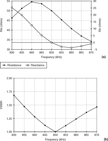
FIGURE 10-9![]()
Common point: (a) impedance, (b) VSWR.
The results are shown in Figure 10-10. Notice that radiation is fairly uniform, perhaps better than might be expected, with the field varying less than half a decibel over the total bandwidth.
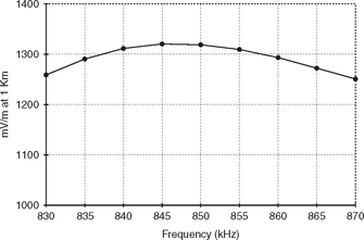
FIGURE 10-10![]()
Field strength at 1 Km versus frequency.
10.4 Bandwidth Conclusions
■ When doing a system analysis, it is important not only to simulate the system realistically but also to simulate the drive signal realistically. In this analysis, a 50-ohm source impedance was simulated to drive the 50-ohm interfaces and the drive to the tower bases was simulated by driving them through the 50-ohm input of their respective ATU network.
■ Low-impedance towers can cause increased parameter variations. These variations must be examined to determine if they are problematic.
■ The transmission lines become mismatched when the frequency varies from the carrier frequency. The length of the transmission line can be of concern when the mismatch causes undesirable impedance transformations.
■ Parameter variations are often smoothed when the multiple paths to the individual towers are combined at the common point. Thus, the performance of the total system is often much better than may be suggested by viewing an ill-performing path to a particular tower.