12.1 Introduction

The previous chapters covered the basic topics that are essential to the design and analysis of MF directional antennas. This chapter adds a few subjects that may not be absolutely necessary, but they are interesting and add some insight to the analysis. Moreover, they are subjects that are not well documented elsewhere; thus, their presentation here fulfills an existing need.

12.2 Parallel Feeds: Network Combiners

When the triangular lattice tower configuration was discussed earlier, the voltage source exciting the tower was placed on a single wire and a spider configuration was used to connect that single-feed wire to each of the three the tower legs. This is a simple arrangement and gives usable results but it has been shown (see Burke and Poggio, “Computer Analysis of the Bottom-fed Fan Antenna,” Report No. 173910, Lawrence Livermore National Labs, August, 1976) that NEC-2 gives a more accurate indication of the self-impedance of the tower when the drive voltage is made up of three separate and equal voltage sources with one source placed on each of the tower legs. See Figure 12-1.

This is equivalent to placing the three sources in parallel so the effective voltage remains the same as that of one source but the total current load is shared by the three sources. Thus, each voltage source sees an impedance that is approximately three times the self-impedance of the tower. Consequently, when the NEC-2 output file displays Impedance under the heading — ANTENNA INPUT PARAMETERS —, it will display three impedances—one for each of the voltage sources. The tower self-impedance must be calculated from the three impedances in parallel. However, since the three impedances will be very nearly equal, a practical self-impedance is simply one-third the value of one of the impedances.

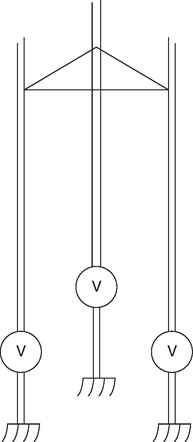
FIGURE 12-1

Multi-source drive on lattice tower.

For most modeling work, using three sources on each tower and handling them as described here does not pose a particular problem.

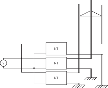
FIGURE 12-2

Drive splitting using networks.

There are instances, however, where it is desired to use the three sources per tower, and at the same time, it is necessary that there be a single drive point. A case in point might be that instance where it is desired to include the antenna-matching network in the model. In that case, three pass-through networks, as shown in Figure 5-2(a) in Chapter 5, may be created by using the NT commands to place all three inputs in parallel on a dummy feed segment containing the source voltage, and then terminating each network output on a separate tower leg. See Figure 12-2.

Because the networks are nonradiating, they will have no effect on the analysis if the dummy feed segment is placed in the far distance and made very short. Should there be reason to suspect that the dummy segment is influencing the result, however, then the LD command can be used to place a large resistance in series with the dummy segment.

12.3 New Structures: The NX Command

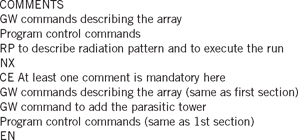
There are occasions where it may be desirable to analyze more than one structure set in a single NEC-2 run. An example of this is the case where it is desired to examine the effect that a parasitic tower may have on an array. A NEC-2 run can be made of the array without the parasitic tower, then another NEC-2 run can be made with the parasitic tower present, and then the two output files compared. However, to eliminate the need to make two separate NEC-2 runs, the comparison can be done in a single NEC-2 run by using the NX command.

When NEC-2 receives the NX command, it is directed to disregard the previously defined structure and to start an analysis of a new structure which will be defined according to the commands that follow. Thus, to make the comparison mentioned above, one would write the NEC-2 input file to describe the array without the parasitic tower. Then, following the EX command, the NX command would be written. The array description would then be copied and pasted following the NX command and the parasitic tower would be added to the array. The input file code would look similar to the following code.

When this input file is run by bnec.exe, the output file will contain two complete sets of output data—one set of data for the array without the parasitic tower, and another set of data for the array with the parasitic tower included.

It is important to recognize that the NX command is simple with only the letters NX written in the first two columns; nothing more. Also, be aware that it is mandatory that the NX command be followed by at least one comment. If there is only one comment, it is written with the CE command. If there is more than one comment, then only the last is written with the CE command, the others are written with CM commands as usual.

Please review the details of the NX command as given in Appendix A.

12.4 Numerical Green's function

Copying and pasting the array data in the previous example is not the most efficient way to accomplish that task. It was used, however, to emphasize the function of the NX command. A more practical scheme is to use the Numerical Green's Function (NGF) to make a structure available without having to repeat the coding of that structure.

The Numerical Green's Function provides the user with the option to generate a structure and save it for later use in the same run, where it may be modified or added to without the expense of having to repeat the coding for the entire structure. This is particularly useful for a big structure that will be analyzed using several modified forms. An example of this is an eight-tower array in which a vehicle has been included in the model and it is desired to determine the effects of the vehicle at several locations.

Perhaps of more immediate application to the broadcaster is the ability of the Numerical Green's Function to take advantage of partial symmetry. In a single run, a structure must be perfectly symmetric for NEC-2 to use symmetry in the solution. Any unsymmetric segments, or ones that lie in the symmetry plane or on the axis of rotation, will prevent the use of symmetry in the analysis. However, partial symmetry may be exploited by creating and running the symmetric part of the model first and writing a NGF file. Then the NX command can be used to create a new structure that is composed of that saved in the NGF file plus the unsymmetric parts that are added to make up the complete structure. This feature is demonstrated in Section 12.5.2, which describes the GR command.

The NGF is used in two steps.

Step 1: The code for the structure to be saved as a NGF file is written as usual. Immediately after the GE command, the frequency, ground parameters, and loading must be set by writing the FR, GN, and LD commands. The EK or KH commands, if applicable, may also be included at that point. Other commands, such as EX and NT, do not affect the NGF and should not be included as part of the NGF file. After the NGF structure has been defined, a WG command is written to cause the NGF data to be saved to a file.

If desired, other commands may follow the WG command (such as to define an excitation and request field calculations) as in a normal run. The WG command should come before XQ, RP, NE, or NH. Also, the FR command must not specify multiple frequencies when a NGF is written.

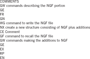
Step 2: Use a NX command to create a new structure that will consist of the saved NGF data plus additions or modifications.

As explained earlier, the command immediately following NX must be a comment. Thereafter, the first geometry command following the CE command must be the GF command to recall the NGF structure that was saved in Step 1 and make it available for inclusion in the total structure. Subsequent structure data commands are then written to define the new structure to be added to the NGF structure.

All types of structure geometry data commands may be used, although GM, GR, GX, and GS will affect the new structure only, not that from the NGF file. While symmetry may have been used in writing the NGF file, it may not be used for the new structures that are used with the NGF file. For connections between the new structure and an NGF structure, the new segment ends must be made to coincide with the NGF segment ends, as would be done in a normal run.

Following the GE command, the program control commands may be used as usual, with the exception that FR and GN commands may not be used again. Recall that the parameters from the FR and GN commands were included in the NGF file. Therefore, following the NX command, those parameters are taken from the NGF file and cannot be changed.

LD commands may be used to load new segments but not segments in the NGF structure since those have already been included. If integers I3 and I4 on a LD command are blank, the command will load all new segments but not NGF segments. If I2, I3, and I4 select a specific NGF segment, the run will terminate with an error message. The effect of loading on NGF segments may be added by using an NT command, since NT (and TL) may connect to either new or NGF segments.

The lines that follow show the form of a NEC-2 input file that uses Numerical Green's Function.

12.5 Ground Screens

Ground screens can be implemented in NEC-2 in two ways: (1) using the GN command to specify a ground screen as one of two media and (2) using the GR command to literally create the ground screen as part of the structure.

12.5.1 The GN Command

The GN command specifies the nature of the ground used in the model and as such, the GN command has the capacity to specify a radial ground screen. But NEC-2 only models the ground screen's effect through an approximation; it does not physically model the wires. As a result, the GN command can only model the ground screen at the origin (x = 0 and y = 0). Therefore, its use is limited to a one-tower analysis. Also, the radial ground screen approximation may not be used with the Sommerfeld"/Norton ground option, which is discussed later. Moreover, the ground screen identified by the GN command cannot be moved by the GM command to create a multitower array because the segments are not identified as geometry. Despite its limitations, however, the GN radial ground screen approximation is very convenient to use when only one tower is being analyzed.

It would be helpful to read the description of the GN command in Appendix A.

A simple NEC-2 input file that creates a ground screen is shown in Listing 12-1. For simplicity, it shows a ground screen over perfect ground, which is a rather impractical notion, but it serves this purpose adequately.

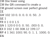
Notice that in addition to displaying the ground-type flag, the GN command now specifies the number of radials in the ground screen (120), the length of the radials (50 meters), and the radius of the wire making up the radials (0.003 meters). Also, the RP command is written to indicate the presence of a ground screen by setting the first integer to 4 (in this case) as opposed to the usual 0. When this NEC-2 input file is run, the presence of the ground screen is noted in the output file just prior to the tabulation of the pattern data.

12.5.2 The GR Command

The GR command is used to advantage when a creating structure containing identical elements spaced symmetrically about the Z-axis. A good example is the ground screen that may consist of as many as 120 identical wire radials equally spaced about the base of the tower. In that case, instead of writing 120 GW commands, it is only necessary to describe one radial with the GW command(s) and then use the GR command to reproduce it 120 times equally spaced about the base of the tower.

Be aware that NEC-2 cannot model wires below the surface of the earth; therefore, the NEC-2 model must be compromised by spacing the wires a small distance above ground. Due consideration must be given the modeling rules, especially those that cause NEC-2 to assume a connection between segment and ground if the spacing is less than 10⁻³ times the length of the segment.

Listing 12-2 is a NEC-2 input file modeling a two-tower array with 120 radial ground screens at each tower. This example serves to demonstrate the GR command, the use of the NGF, and the NX command.

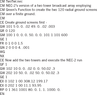
In summary, the file exploits the symmetry of the 120 radial ground screens by generating the screens separately and adding the towers after the screens are complete. Figure 12-3 demonstrates the principle.

Refer to Listing 12-2 to see that the two parts are generated and combined by generating one ground screen at the origin using the GR command to replicate the single radial that was described by the preceding GW command. Once created at the origin, the total ground screen is duplicated at a location 50 meters north by using the GM command. Following that, the GE, FR, and GN commands define the appropriate parameters. Then all are saved by writing them to a NGF file via the WG command.

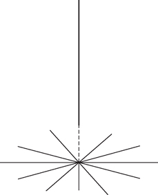
FIGURE 12-3

Monopole added to ground screen

Because NEC-2 cannot model wires underground, the ground screen in this example has been placed 0.02 meters above ground. Remember, however, that if the radials are placed too close to the ground, NEC-2 will try to connect the radial wires to ground and will reject the input with an error message. This is not a concern when using NEC-4 because the radial wires may be placed underground with that code.

The NX command then starts a new structure that will be created by recalling the two ground screens with the GF command and then adding a tower to each ground screen, as described by the next two GW commands.

Following the end of the geometry definition are the excitation and radiation pattern commands used in the conventional way.

When a finite ground is used, NEC-2 shows zero radiation at ground level, so the RP command must call for a pattern at some small angle above the horizon. In this example, theta has been arbitrarily specified as 80° (10° above the horizon), although that may be a bit large.

Refer to Appendix A to study the details of the commands used in this example. Notice especially that the number in the second field of the GR command specifies how many radials are to be created. This number is the total number of radials to be created including the one described by the GW command. For example, if a total of 120 radials is desired and one is described by the GW command, then 120 would be entered in the GR command, not 119. The total number of times that the structure can be repeated is limited by array dimensions in the NEC-2 program. In the NEC-2 files available on the Internet, the limit is 16 times. However, the program associated with this book, bnec.exe, has been modified to accept 120 radials, in keeping with the usual broadcast practice. If this modification causes bnec.exe to exceed the memory limits of the computer, use bnec3k.exe or download a suitable NEC-2 program from the Internet.

The GR command should never be used when there are segments on the Z-axis or crossing the Z-axis since overlapping segments would result. Placement of nonradiating networks or sources does not affect the use of the GR command, however.

The reader is encouraged to enter the NEC-2 input file of Listing 12-2 and to run the NEC-2 analysis. It is useful to know that the input file twotwr.nec takes almost 2 minutes to run using bnec.exe on a 2.7-GHz machine. Each radial in the ground screen has 5 segments and there are 120 radials in each ground screen, so the two ground screens have a total of 1200 segments. Then each of the two towers has 10 segments, so there are a total of 1220 segments in the model. This large number of segments exceeds the capability of NECMOM.EXE; thus, the calculated field ratios cannot be determined using the furnished software.

The output file will contain the equivalent of two regular NEC-2 output files—one for the NGF structure containing ground screens only and another containing ground screens plus towers. You are encouraged to study this output file carefully.

12.6 Finite Ground

For the most part, specifying a perfectly conducting ground for the NEC-2 analysis of a broadcast directional array simplifies the task and gives satisfactory results. The elaborate ground screens used with broadcast antennas and the fact that the surface impedance at the center of a ground screen is zero causes the calculated impedance and current distribution using the ground screen to be equivalent to that of a perfectly conducting ground. This encourages one to choose the simpler perfect ground rather than a finite ground for most broadcast analysis.

There are, however, occasions that make it necessary to model the system using a finite ground. This section introduces the subject of finite grounds but the coverage is by no means complete in itself.

NEC-2 uses two procedures in addressing a finite ground. The Reflection Coefficient Approximation (RCA) is simple and sufficiently accurate for those applications where horizontal conductors are not too near the ground. The Sommerfeld/Norton method is more accurate in general and has more application near the ground but it is less convenient to use and uses more computer time.

12.6.1 Reflection Coefficient Approximation

The Reflection Coefficient Approximation computes the radiated field over a real ground by including the field of the image structure as modified by a reflection coefficient determined by the surface impedance of the ground at the spectral point. The RCA can only be used with horizontal wires that are not too close to the ground, with reasonable results being obtained when those wires are more than 0.1 to 0.2 wavelengths above ground.

The use of the RCA is selected by setting I2 = 0 in the GN command and specifying the ground dielectric constant and conductivity. For example,

12.6.2 Sommerfeld/Norton Analysis

The more accurate Sommerfeld/Norton ground method uses exact solutions for fields in the presence of the specified ground and is more accurate for horizontal wires that are closer to the ground. It is less convenient to use, however, not only because it is more time consuming when running but also because it requires a look-up table that must be created prior to the NEC-2 run. Rather than make certain laborious calculations when the Sommerfeld/Norton method is used, NEC-2 looks to a grid of values in a look-up table of previously calculated results. It interpolates within the grid for values as required.

For most NEC-2 versions available on the Internet, it is necessary for the user to create the look-up table by running an auxiliary program named SOMNEC prior to making the NEC-2 calculation. SOMNEC accepts user input of relative dielectric constant, ground conductivity and frequency and then writes an output as a binary file, which NEC-2 reads.

In the software associated with this book (see Appendix C), however, SOMNEC has been incorporated directly into the NEC-2 program, bnec.exe. It is not necessary for the user to create the look-up table file because bnec.exe calculates the values internally as needed.

When the Sommerfeld/Norton ground is used, the NEC-2 output file states that fact under the heading — ANTENNA ENVIRONMENT — in addition to listing the specified dielectric constant and conductivity.

The use of Sommerfeld/Norton is selected by setting I2 = 2 in the GN command and specifying the ground dielectric constant and conductivity.

For example,

Refer to the GN command in Appendix A for more information about the Sommerfeld/Norton ground.