Chapter 8
Local Filters
Local filters extend point operations by having the output be some function of the pixel values within a local neighbourhood or window:
where W is the window or local neighbourhood centred on ![]() , as illustrated in Figure 8.1. The window can be any shape or size, but is usually square, W × W pixels in size, with W odd so that the window centre is well defined. As the window is scanned through the input image, each possible position generates an output pixel according to Equation 8.1. Again, f is any function, with the particular function determining the type of filter. Since the output depends not on only the input pixel but also its local context, filters can be used for noise removal or reduction, edge detection, edge enhancement, line detection and feature detection.
, as illustrated in Figure 8.1. The window can be any shape or size, but is usually square, W × W pixels in size, with W odd so that the window centre is well defined. As the window is scanned through the input image, each possible position generates an output pixel according to Equation 8.1. Again, f is any function, with the particular function determining the type of filter. Since the output depends not on only the input pixel but also its local context, filters can be used for noise removal or reduction, edge detection, edge enhancement, line detection and feature detection.
Figure 8.1 A window filter. The shaded pixels represent the input window located at × that produces the filtered value for the corresponding location in the output image. Each possible window position generates the corresponding pixel value in the output image.

The software approach to filtering has both the input and output images stored in frame buffers. The algorithm iterates for each output pixel, retrieving the pixels within the window in the input image and applying the filter function. In this form, the algorithm is ultimately limited by the bandwidth of the input memory.
Any acceleration of filtering must exploit the fact that each pixel is used in multiple windows. With stream processing, this is accomplished through caching pixels as they are read in to enable them to be reused in later window positions.
Pixel caching for stream processing of a W × W filters requires a series of W − 1 row buffers, as described in Section 5.2.3. Scanning the window through the image is equivalent to streaming the image through the window. The row buffers can either be placed in parallel with the window or, since the window consists of a set of shift registers, in series with the window as shown in Figure 8.2. Computationally they are equivalent. The parallel row buffers need to be slightly longer (the full width of the image) but have the advantage that they are kept independent of the window and filter.
Figure 8.2 Row buffers. Left: in parallel with window; right: in series with window.

Variations on this stream access pattern are also possible. If the resources are limited and the row buffer is too long for the available memory, then the image may be scanned down the columns rather than across the rows. Alternatively, the image may be partitioned and processed as a series of vertical strips (Sedcole, 2006), as illustrated in Figure 8.3. In the latter case, there is a small overhead because to process the complete image the vertical strips will have to overlap by W − 1 pixels.
Figure 8.3 Access patterns for stream processing.

Conversely, if additional resources and memory bandwidth are available, the image may be partitioned with multiple filters operating in parallel. However, rather than partition the image as illustrated on the right in Figure 8.3, it can be more efficient to simultaneously process multiple adjacent rows (Draper et al., 2003). This requires multiple pixels to be input per clock cycle and exploits the fact that the windows for vertically adjacent outputs overlap significantly, as can be seen in Figure 8.4. This is partially unrolling the vertical scan loop through the image. Note that the number of row buffers is unchanged. For an unroll factor of k (processing k rows of pixels in parallel) the combined window size is ![]() . Of this, k rows of data are streamed in from memory in parallel, so the remaining W − 1 rows must come from row buffers. These buffers are arranged with a pitch of k rather than simply being chained. The parallel implementation will require k copies of the filter function. However, with some filters, the overlap in windows can even enable some of the filter function logic to be shared (Lucke and Parhi, 1992), reducing the resource requirements further.
. Of this, k rows of data are streamed in from memory in parallel, so the remaining W − 1 rows must come from row buffers. These buffers are arranged with a pitch of k rather than simply being chained. The parallel implementation will require k copies of the filter function. However, with some filters, the overlap in windows can even enable some of the filter function logic to be shared (Lucke and Parhi, 1992), reducing the resource requirements further.
Figure 8.4 Partially unrolling the loop vertically, streaming in multiple rows in parallel.

Partially unrolling the scan loop vertically will require reading pixels from k rows of the image. However, these pixels are not usually stored together in memory, requiring an awkward memory access pattern. Pixels are more likely to be packed in memory, so it may be preferable to read multiple horizontal pixels simultaneously. Figure 8.5 demonstrates a partial horizontal unrolling of the scan loop. This time k horizontally adjacent pixels are processed simultaneously, making the combined window size ![]() . This also requires the shifting pitch of the window registers to be k pixels. W − 1 row buffers are still required, but their aspect ratio must be changed to provide the wider combined data. Again, k copies of the filter function are required, although for some functions some of the filter logic may be able to be shared.
. This also requires the shifting pitch of the window registers to be k pixels. W − 1 row buffers are still required, but their aspect ratio must be changed to provide the wider combined data. Again, k copies of the filter function are required, although for some functions some of the filter logic may be able to be shared.
Figure 8.5 Partially unrolling horizontally, streaming multiple pixels each clock cycle.
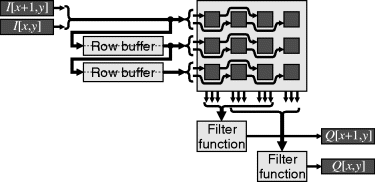
Although the internal memory of most FPGAs is dual-port (only simple dual-port is required for circular memory-based row buffers), it is possible to cache the input rows using only single-port memory. This requires W buffer memories, with the input being written to one buffer and row 0 of the window, while the other rows of the window are read from other row buffers as shown in Figure 8.6. Table 8.1 shows the corresponding control for a 3 × 3 window. The state is easiest implemented as a ring counter, directly controlling the read/write signals to the memories and the multiplexers.
Figure 8.6 Filtering with single-port row buffers (see Table 8.1 for the control sequence).

Table 8.1 Control for single-port row buffer in Figure 8.6

One problem with filtering is managing what happens when the window is not completely within the input image (Bailey, 2011b). Very few papers consider these boundary conditions – the design to handle them properly can take more effort than to manage the normal case where all of the data is available. For some solutions, the logic required to handle the boundary cases can be just as much or more than the regular window logic. There is a wide range of solutions that can be considered:
- The output could be left uncalculated for the boundary pixels. The output image would become
 pixels smaller. In many applications and with a small window size this would not be a problem.
 - The filter function could be modified to work with the smaller window when part of the window extends beyond the boundary of the image. For many filters, this is not an option and, where it is, the logic requirements can grow rapidly to manage the different cases.
- The input image could be made larger. This requires manufacturing
 pixel values beyond each border of the image so that there is sufficient data to fill the window to produce a full-sized image at the output. An original
  image is extended to produce the
  input image that is processed. The following options describe different techniques for extending the input image in order of complexity.
 - The input stream can just be wrapped. This is equivalent to ignoring the problem and simply processing the
 image. The pixels at the end of a row are immediately followed by the pixels at the start of the next row. Similarly, the last row of one frame is immediately followed by the first row of the next frame. Since the opposite edges of an image are not likely to be related in most applications, the border pixels are likely to be invalid. However, the advantage over the first case above is that output pixels are produced and the output image is the same size as the input.
 - A predefined value could be used for the pixels outside the image. This could be black (0), white, or some other value depending on the type of filter and the expected scene.
- The pixel values on the border of the image could be duplicated, assigning the value to that of the nearest available pixel. This is effectively nearest neighbour extrapolation. This approach has been used with median and rank filters (Choo and Verma, 2008).
- The previous extension made the pixels outside the image flat. With some filter functions, this may result in undesired artefacts around the edge. An alternative is to mirror the rows and columns just inside the border to the outside of the image. Mirroring is commonly used with wavelet filters. There are two approaches to mirroring that have been used. One mirrors using the edge of the image, duplicating the border pixels (Kurak, 1991), and the other mirrors from the border row, without duplicating the border pixels (McDonnell, 1981; Benkrid et al., 2003a). These approaches are compared in Figure 8.7.
Figure 8.7 Edge extension schemes. Left: border pixel duplication; centre: mirroring with duplication; right: mirroring without duplication.

Whatever extension method is used, it is easier to apply it between the row buffering and forming the filter window than to attempt to modify the filter function to handle the boundary conditions. Specific mechanisms for achieving this are described after discussing the priming and flushing requirements of filter pipelines.
It is necessary to load a whole window of data before the output starts. The time required to prime the filter and fill the row buffers for a W × W window is the time for loading W − 1 complete rows of ![]() pixels plus an additional W pixels. Therefore:
pixels plus an additional W pixels. Therefore:
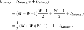
However, at the top of the image, half of these rows are outside the boundary of the image. The latency of the filter is the time from when a pixel is input to when the corresponding output pixel is produced, and can be broken into two components. The first is that of the windowing operation and the second is the latency of the filter function itself. The latency of windowing is the time from when the centre pixel is loaded to when the last pixel is loaded for that window position, enabling the output to be calculated. This gives:
If the system is sink-driven, then it is necessary to start the filtering at least this length of time before the first data is required on the output. The filter must also be clocked for this many clock cycles after the last data is input to flush the contents of the filter. Note the times of Equations 8.2 and 8.3 are further complicated if the input stream has additional horizontal and vertical blanking intervals.
Part of priming the filter window includes loading the extended input image (beyond the borders of the original image). Consider the case of boundary replication – the first and last rows must be loaded ![]() times, and similarly the first and last pixels on each row. Rather than explicitly reload them, it is possible to reuse the loaded values using the scheme of Figure 8.8. As the first pixel of each row is streamed in, the value is loaded into all of the shift register stages on the input. This allows the first pixel to be replicated an additional
times, and similarly the first and last pixels on each row. Rather than explicitly reload them, it is possible to reuse the loaded values using the scheme of Figure 8.8. As the first pixel of each row is streamed in, the value is loaded into all of the shift register stages on the input. This allows the first pixel to be replicated an additional ![]() times. The rest of the stream also passes through the input shift register to enable the whole row to be streamed continuously. As the last pixel of the row is loaded into the window, the last shift register stage is fed back replicating the last pixel of the row. At this stage the first row buffer contains the whole first row, including the duplicated pixels at the boundaries. This row is recirculated to the input
times. The rest of the stream also passes through the input shift register to enable the whole row to be streamed continuously. As the last pixel of the row is loaded into the window, the last shift register stage is fed back replicating the last pixel of the row. At this stage the first row buffer contains the whole first row, including the duplicated pixels at the boundaries. This row is recirculated to the input ![]() times through the R input of the multiplexer, repeating the first row as necessary. Then the remainder of the image is streamed in, with the last row repeated as before while flushing data out of the window.
times through the R input of the multiplexer, repeating the first row as necessary. Then the remainder of the image is streamed in, with the last row repeated as before while flushing data out of the window.
Figure 8.8 Priming the filter. Row and pixel replication at the boundaries.
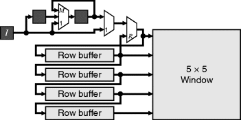
A similar approach may be used for mirroring the input, although the multiplexing gets a little more complex. One disadvantage of this approach is that it requires at least ![]() clock cycles to process the whole image, and the row buffers need to be slightly longer than one row. However, since only
clock cycles to process the whole image, and the row buffers need to be slightly longer than one row. However, since only ![]() pixels are loaded in and
pixels are loaded in and ![]() pixels are output, it should be possible to process pixels continuously, without the delays associated with repeating pixels and rows. An approach that does that, using mirroring without duplication, for a 5 × 5 window is demonstrated in Figure 8.9 (Bailey, 2011b).
pixels are output, it should be possible to process pixels continuously, without the delays associated with repeating pixels and rows. An approach that does that, using mirroring without duplication, for a 5 × 5 window is demonstrated in Figure 8.9 (Bailey, 2011b).
Figure 8.9 Priming the filter with mirroring and no additional delay between rows.

The operation of this is a little more complex. Firstly consider the operation along a row. In normal operation (in the centre of the image) the bottom row of shift registers is used to shift the pixels along. At the end of the row, the first pixels of the next row are clocked into the top row of shift registers. Meanwhile, the appropriate pixel from within the window is fed back to the start of the window to give the mirroring. The labels on the input multiplexer refer to the second last (−2) and last (−1) positions of the window on the row. On the next clock cycle, the window should correspond to the first position on the next row. While flushing the end of one row, the initial pixels required to prime the window for the next row have been loaded. These are now transferred to the appropriate window registers (through multiplexer inputs labelled 1) to give the mirrored window values. Note that no clock cycles have been lost here – the window transitions from the last position on one row directly to the first position on the next row.
A similar procedure could be used for transitioning from the bottom of one image to the top of the next. However, this would require two extra row buffers to perform the counterpart of the preload registers along the row. Instead, the outputs from the row buffers are routed directly to the corresponding rows of the window. Mirroring requires feeding back the data at the bottom of the window; multiplexer inputs −2 and −1 refer to the second last and last rows of the image respectively. On the first and second rows of the new image, multiplexer inputs 1 and 2 respectively feed forward the row buffered and input data to reflect the mirroring.
This Section has shown how row buffers can be used to cache the data associated with local filters. Each pixel is only loaded once, with the value reused for all of the window positions that require it. A throughput of one pixel per clock cycle can be maintained (or higher if partially unrolling the raster scan). It is also possible to process the borders of the image without introducing additional latency with only a small amount of additional control logic.
The filter function for a linear filter is a weighted sum of the pixel values within the window.
The particular set of weights is sometimes called the filter kernel, with the filter function determined by the kernel used. Linear filtering is equivalent to performing a two-dimensional convolution with the flipped kernel, ![]() . Since the Fourier transform of a convolution is a product of the respective Fourier transforms (Bracewell, 2000), the operation of linear filters can be also be considered from their effects in the frequency domain. This is considered further in Chapter 10.
. Since the Fourier transform of a convolution is a product of the respective Fourier transforms (Bracewell, 2000), the operation of linear filters can be also be considered from their effects in the frequency domain. This is considered further in Chapter 10.
In signal processing terminology, the filters described by Equation 8.4 are finite impulse response filters. Recursive, infinite impulse response filters can also be used; these use the previously calculated outputs in addition to the inputs to calculate the current output:
(8.5) ![]()
By necessity, ![]() must be zero for the pixels that have not been calculated yet. While recursive filters may be used to implement some finite impulse response filters (for example box filters described below), they are otherwise not often used in image processing. The nonlinear phase response results in a directional smearing of information within the image. To avoid this, it is necessary to apply each filter twice, once with a top-to-bottom, left-to-right scan pattern, and again with a bottom-to-top, right-to-left scan pattern. This makes such filters harder to pipeline, although for a given frequency response, infinite impulse response filters require a significantly smaller window (Mitra, 1998). Only finite impulse response filters are discussed further in this Section.
must be zero for the pixels that have not been calculated yet. While recursive filters may be used to implement some finite impulse response filters (for example box filters described below), they are otherwise not often used in image processing. The nonlinear phase response results in a directional smearing of information within the image. To avoid this, it is necessary to apply each filter twice, once with a top-to-bottom, left-to-right scan pattern, and again with a bottom-to-top, right-to-left scan pattern. This makes such filters harder to pipeline, although for a given frequency response, infinite impulse response filters require a significantly smaller window (Mitra, 1998). Only finite impulse response filters are discussed further in this Section.
8.2.1 Noise Smoothing
One of the most common filtering operations is to smooth noise. The basic principle behind noise smoothing is to use the central limit theorem to reduce the noise variance. With only one image, it is not possible to average with time as was used in Section 6.2.1. Instead, adjacent pixels are averaged. To avoid the output value from being different from the input in uniform regions of the image, a noise smoothing filter requires:
(8.6) ![]()
Most images have their energy concentrated in the low frequencies, with the high frequencies containing information relating to fine details and edges (wherever the pixel values are changing quickly). Random (white) noise has a uniform frequency distribution. Therefore, a low pass filter will remove the most noise while having the least impact on the energy content of the image. Unfortunately, in attenuating the noise, the high frequency content of the image is also attenuated, resulting in blur.
With linear filters, their effect on the noise and the image content can be analysed separately. Assuming that the noise is independent for each pixel, then from Equation 6.16 the best improvement in variance for a given size window will result if the weights are all equal. A larger width window will result in more noise smoothing. These noise suppression effects can be clearly seen in Figure 8.10, where an image with artificially added noise is filtered.
Figure 8.10 Linear noise smoothing filters.
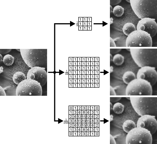
Spatial averaging will result in a loss of fine detail and a blurring of edges. Unfortunately, these effects will become worse with increased noise smoothing. Therefore, there is a trade-off between blurring and noise suppression, as is also seen in Figure 8.10.
The Fourier transform of a uniform filter is a sinc function, which has poor sidelobe performance at high frequencies. These sidelobes mean that significant high frequency noise still remains after filtering. This is apparent in the fine textured region in the centre image in Figure 8.10. A better low pass filter can be obtained by rolling off the weights towards the edge of the kernel. While the noise variance will be higher, there is better attenuation of the high frequency noise and fewer filtering artefacts.
A commonly used filter has Gaussian weights:
(8.7) ![]()
where ![]() is the standard deviation or equivalent radius of the filter. Note that the Gaussian weights never actually go to zero, so a practical implementation will require truncating the weights within a finite rectangular region. The filter width, W, should generally be greater than about
is the standard deviation or equivalent radius of the filter. Note that the Gaussian weights never actually go to zero, so a practical implementation will require truncating the weights within a finite rectangular region. The filter width, W, should generally be greater than about ![]() and, if accuracy is important, then
and, if accuracy is important, then ![]() . With truncation, the kernel coefficients may require rescaling to make the total equal to one. The filter in the bottom row of Figure 8.10 corresponds to
. With truncation, the kernel coefficients may require rescaling to make the total equal to one. The filter in the bottom row of Figure 8.10 corresponds to ![]() .
.
One application of Gaussian filtering is to obtain a scale–space representation of an image (Lindeberg, 1994). Filtering by a series of Gaussian filters with successively larger standard deviations will remove from the image features of increasing size or scale.
8.2.2 Edge Detection
Edge detection is another common application of filtering. At the edges of objects, there is often a change in pixel value, reflecting the contrast between the object and the background, or between two objects. Since the edge is characterised by a difference in pixel values, a differencing filter can be used to detect edges. Differencing is sensitive to noise, so the top filter in Figure 8.11 averages vertically (to give noise smoothing) while differencing horizontally to detect vertical edges. Note that differencing like this will only detect edges of particular orientation. Alternatively, since the edges contain high frequency information (this was lost through the low pass noise smoothing filter), a high pass filter can be used to detect edges of all orientations. The main limitation of high pass filters is their strong sensitivity to noise (see the middle filter of Figure 8.11).
Figure 8.11 Linear edge detection filters. Top: vertical edge detection; centre: high pass filter; bottom: Laplacian of Gaussian filter. The output images are offset to show negative values.
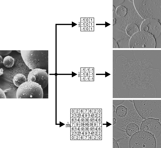
The noise sensitivity can be improved significantly by first filtering the image with a Gaussian filter. However, there is a trade-off between accurate detection (improves with smoothing) and accurate localisation (deteriorates with smoothing) (Canny, 1986). With the smoothed image, the peaks of the first derivative will correspond to the location of the edges. These can either be found directly or by finding the zero crossings of the second derivative. (Note that finding the peaks or zero crossings requires a nonlinear filter, which will be described in the next Section.)
With linear filters, it does not matter whether the derivatives are taken before or after smoothing. Indeed they can even be combined with the smoothing to give a single filter. With the first derivative, there are two filters for derivatives in each of the x and y directions. The corresponding weights are:
(8.8) 
Using the Laplacian for the second derivative makes the second derivative filter (Laplacian of Gaussian or LoG filter) (Marr and Hildreth, 1980):
(8.9) ![]()
The LoG filter can be used to detect edges of all orientations. It is effectively a band-pass filter, where the standard deviation, ![]() , controls the centre frequency or the scale from a scale–space perspective, at which edges are detected. The bottom image of Figure 8.11 shows the Laplacian of Gaussian filter with
, controls the centre frequency or the scale from a scale–space perspective, at which edges are detected. The bottom image of Figure 8.11 shows the Laplacian of Gaussian filter with ![]() . If the Gaussian and Laplacian operations are separated, then one of the Laplacian kernels in Figure 8.12 may be used.
. If the Gaussian and Laplacian operations are separated, then one of the Laplacian kernels in Figure 8.12 may be used.
Figure 8.12 Filter kernels for a Laplacian filter.

A filter with a similar response to the LoG filter is the difference of Gaussians (or DoG filter). It is formed by subtracting the output of two Gaussian filters with different standard deviations:
(8.10) ![]()
where ![]() is the ratio of standard deviations of the two Gaussians. This corresponds closely to the receptive field response within the human visual system (Wilson and Giese, 1977).
is the ratio of standard deviations of the two Gaussians. This corresponds closely to the receptive field response within the human visual system (Wilson and Giese, 1977).
Note that the weights for an edge detection filter should sum to zero, so that the response is zero for regions of uniform pixel value. For edge detection, the weights can be multiplied by an arbitrary constant, since the edges correspond either to the positions of the maximum derivatives, or the locations of the zero crossings of the Laplacian.
8.2.3 Edge Enhancement
An edge enhancement filter sharpens edges by increasing the gradient at edges. In this sense it is the opposite of edge blurring, where the gradient is decreased by attenuating the high frequency content. Edge enhancement works by boosting the high frequency content of the image. One such filter is shown in Figure 8.13. A major limitation of the high frequency gain is that any noise within the image will also be amplified. This cannot be easily avoided, so linear edge enhancement filters should only be applied to relatively noise-free images. Over-enhancement of edges can result in ringing, which will become more severe as the enhancement is increased.
Figure 8.13 Linear edge enhancement filter.

The weights of an edge enhancement filter must sum to one to avoid changing the global contrast of the image.
8.2.4 Linear Filter Techniques
Although most of the examples shown in this Section are 3 × 3 filters, the techniques readily extend to larger filter sizes. The obvious implementation of a linear filter is illustrated in Figure 8.14, especially if the FPGA has plentiful multiplication or DSP blocks. Each pixel within the window is multiplied in parallel by the corresponding filter weight and then added. Note that the bottom right window position is the oldest pixel and corresponds to the top left pixel within the image in the image. The filter weights are shown here as constants, but could also be programmable and stored in a set of registers.
Figure 8.14 Direct implementation of linear filtering.
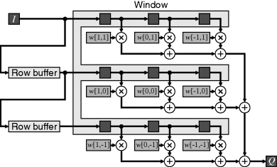
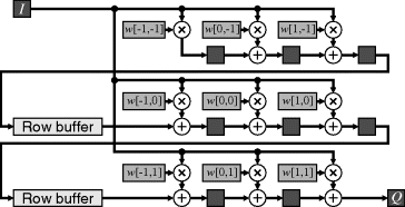
The propagation delay through the multiplication and adders may exceed the system clock cycle and require pipelining. Since each input pixel contributes to several pixels, rather than delaying the inputs and accumulating the output, the transpose filter structure performs all the multiplication with the input and delays the product terms (Mitra, 1998). The transpose filter structure does this by feeding data through the filter backwards (swapping the input and the output) and swapping summing junctions and pick-off points. This is applied to each row in Figure 8.15, and to the whole window (Benkrid et al., 2003a) in Figure 8.16. The advantage of the transposed structures is that the output is automatically pipelined. When transposing the whole window, it is necessary to cache the partial sums using row buffers until the remainder of the window appears. Depending on the filter coefficients, these partial sums may require a few guard bits to prevent accumulation of rounding errors. The row buffers, therefore, may need to be a few bits wider than the input pixel stream. The transposed filter structures may also require a little more effort to manage the image boundaries, although that can also be incorporated into the filter structure (Benkrid et al., 2003a).
Figure 8.15 Pipelined linear filter. Note the different order of coefficients to Figure 8.14 because the transpose filter structure is used for each row.
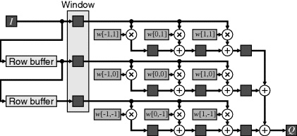
Figure 8.16 Transposed implementation of linear filtering. Note the changed coefficient order.
There are several techniques that may be used to simplify and reduce the logic required by linear filters. Many filters are symmetric, therefore many of their filter coefficients share the same value. If using the direct implementation of Figure 8.14, the corresponding input pixel values can be added prior to the multiplication. Alternatively, since each input pixel is multiplied by a number of different coefficients, the input pixel value can be multiplied by each unique coefficient once, with the results cached until needed (Porikli, 2008). This fits well with the transposed implementation of Figure 8.16. In both cases, the number of multipliers is reduced to the number of unique coefficients.
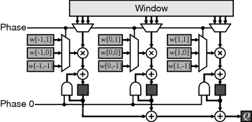
If using a relatively slow clock rate, and hardware is at a premium, then significant hardware savings can often be made by doubling or tripling the clock rate but keeping the same data throughput. The result is a multiphase design which enables expensive hardware (multipliers in the case of linear filters) to be reused in different phases of the clock. This is shown for a three-phase system in Figure 8.17. With the accumulator, a 0 is fed back in phase zero to begin the accumulation for a new pixel.
Figure 8.17 Reducing the number of multipliers by using a higher clock speed.
Many useful filters are separable:
(8.11) ![]()
This means that a two-dimensional filter may be decomposed into a cascade of two one-dimensional filters: a 1 × W filter operating on the columns and a W × 1 filter operating on the rows. This will reduce the number of both multiplications and associated additions from W2 to 2W. Note that the column filter does not require a separate pass through the image. It, too, can be streamed by replacing the pixel delays within the window by row buffers, as shown in Figure 8.18. This is effectively implementing the filters for each column in parallel, but sequentially stepping the filter function from one column to the next as the data is streamed in. Consequently, the row and column filters may be directly pipelined.
Figure 8.18 Converting a row filter to a column filter by replacing pixel delays with row buffers.

While not all filters are directly separable, even arbitrary two-dimensional filters may be decomposed as a sum of separable filters (Lu et al., 1990; Bouganis et al., 2005)
(8.12) ![]()
through singular value decomposition of the filter kernel. The vectors associated with the k largest (significant) singular values will account for most of the information within the filter. With such a decomposition, the column filters should be implemented before the row filters to enable a single set of row buffers to be used for all the parallel filters. For a similar reason, the transpose filter structure cannot be used for the column filters, although it may be used for the row filters. Such a decomposition can give savings if ![]() , which will be the case if the original filter is symmetrical either horizontally or vertically.
, which will be the case if the original filter is symmetrical either horizontally or vertically.
Also worth considering are series decompositions of filters. The kernel of a composite filter is the convolution of the kernels of the constituent filters:
(8.13) 
A common example of this is approximating a Gaussian filter by repeated application of a rectangular box filter. For k repetitions of a window of width W, the standard deviation of the resultant approximate Gaussian is:
(8.14) ![]()
For many applications, three or four repetitions will provide a sufficiently close approximation to a Gaussian filter.
Of course, when implementing constant coefficient filters, if any of the coefficients is a power of two, the corresponding multiplication is a trivial shift of the corresponding pixel value. Such shifts can be implemented without logic. If not using multiplier blocks, the multiplications may be implemented with shift and add algorithms. For any given coefficient, the smallest number of shifts and adds (or subtracts) is obtained by using the canonical signed digit representation for the coefficients. Further optimisations may be obtained by identifying common subexpressions and factorising them out (Hartley, 1991). For example, 165 = 101 001 012 requires three adders for a canonical signed digit multiplication, but only two by factorising as 5 × 33 (= 1012 × 1 000 012). A range of techniques has been developed to find the optimal (in some sense) factorisation and arrangement of terms (Dempster and Macleod, 1994; Potkonjak et al., 1996; Martinez-Peiro et al., 2002; Al-Hasani et al., 2011).
A simple example will illustrate the power of these techniques. Consider a 21 × 21 Gaussian smoothing filter with ![]() . A direct implementation would require 441 multipliers and 440 adders. Representing the coefficients with fixed-point numbers with resolution of 2−16 has the coefficients in the range from 0 to 1160, requiring 11 bits for the central few coefficients. Of the coefficients, 40 of them are zero, so do not need to be multiplied or added in. This reduces the number of adders to 400. Of the coefficients, 96 are direct powers of two (1, 2, 4 and 8); these also will not require multipliers but will still require adders. Since the filter is symmetric, most of the coefficients will be used four or eight times. This can be exploited by adding the corresponding pixel values first and then multiplying by the coefficient. Since there are 40 unique coefficients (not counting the zero or powers of two), this reduces the number of multipliers to 40, although 400 adders are still required. A further 10 of the coefficients can be represented as the sum or difference of two powers of two. This allows those multiplications to be performed by a single addition rather than a multiplication. The number of operations is then 30 multiplications and 410 additions.
. A direct implementation would require 441 multipliers and 440 adders. Representing the coefficients with fixed-point numbers with resolution of 2−16 has the coefficients in the range from 0 to 1160, requiring 11 bits for the central few coefficients. Of the coefficients, 40 of them are zero, so do not need to be multiplied or added in. This reduces the number of adders to 400. Of the coefficients, 96 are direct powers of two (1, 2, 4 and 8); these also will not require multipliers but will still require adders. Since the filter is symmetric, most of the coefficients will be used four or eight times. This can be exploited by adding the corresponding pixel values first and then multiplying by the coefficient. Since there are 40 unique coefficients (not counting the zero or powers of two), this reduces the number of multipliers to 40, although 400 adders are still required. A further 10 of the coefficients can be represented as the sum or difference of two powers of two. This allows those multiplications to be performed by a single addition rather than a multiplication. The number of operations is then 30 multiplications and 410 additions.
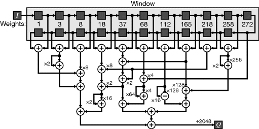
A further observation is that the Gaussian filter is separable. This allows the 21 × 21 filter to be implemented as cascade one-dimensional Gaussian filters (1 × 21 and 21 × 1). The fixed-point coefficients with a resolution of 2−11 are shown along the top of Figure 8.19. Each one-dimensional filter would require nine multiplications (because of symmetry and two coefficients are powers of two) and 20 additions. A further six coefficients can be represented as a sum or difference of two powers of two, reducing the requirements to three multiplications and 25 additions (one addition can be removed through common subexpression elimination: 272 = 4 × 68). The remaining three multiplications can also be eliminated by reusing common subexpressions, in the form of a shifted sum of two existing coefficients (37 = 2 × 18 + 1; 165 = 37 + 128; 218 = 8 × 18 + 2 × 37) allowing even those multipliers to be replaced with single additions. Therefore, the complete 21 × 1 filter can be implemented with only 28 additions, as demonstrated in Figure 8.19. A similar filter can be used for the vertical filter, replacing each the register in the chain across the top with a row buffer.
Figure 8.19 Adder only implementation of a 21 × 1 Gaussian filter with ![]() .
.
With the increasing prevalence of high speed pipelined multipliers within FPGAs, the need for such decompositions has diminished somewhat in the last few years. The optimised hardware multipliers are hard to out-perform with the relatively slow adder logic of the FPGA fabric (Zoss et al., 2011).
Other decompositions and approximations are also possible, especially for large windows. For example, Kawada and Maruyama (2007) approximate large circularly symmetric filters by octagons and rely on the fact that the pixels with a common coefficient lie on a set of lines. As the window scans, the total for each octagon edge is updated to reflect the changes from one window position to the next.
A simpler version of this can be applied to averaging using a rectangular window with equal weights (McDonnell, 1981). Firstly, a large rectangular window is separable, allowing the filter to be implemented as a cascade of two one-dimensional filters. Secondly, the equal weights make the filter amenable to a recursive implementation:
(8.15) 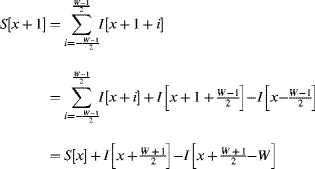
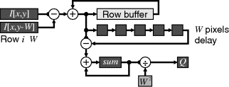
which reduces the one-dimensional filter to a single addition and subtraction regardless of the size of the window. The same recursive mechanism may also be used for the column filter. An input pixel is then only required twice, once when it first enters the window and again when it leaves the window. For large windows, a large number of row buffers are required to cache the input for its second access. Therefore, if the input stream is from a frame buffer which has sufficient bandwidth to stream from two rows simultaneously, the row buffering requirements can be reduced significantly, with only the current column sum buffered. Such an implementation for a W × W box average is illustrated in Figure 8.20.
Figure 8.20 Efficient implementation of a ![]() box average filter.
box average filter.
While the theory behind linear filters is well established and the filters are relatively simple to implement, restricting f in Equation 8.1 to a linear combination of the input values has some significant limitations (Bailey et al., 1984). In particular, the filters have difficulty distinguishing between legitimate changes in pixel value (for example at an edge) from undesirable changes resulting from noise. Consequently, linear filters will blur edges while attempting to reduce noise, or be sensitive to noise while detecting edges or lines within the image.
Linear filters may be modified to improve their characteristics, for example by making the filter weights adaptive, or dependent on the image content. The simplest of these are trimmed filters, which omit some pixels within the window from the calculation. While the mean possesses good noise reduction properties, it is sensitive to outliers. A trimmed mean will discard the outliers by discarding the extreme pixels and calculate the mean of the remainder (Bednar and Watt, 1984). With a heavy tailed noise distribution, this can give an improvement in signal-to-noise ratio. A related application is smoothing noise without significantly blurring edges; it is desirable to average the pixel values only from one side of the edge. By selecting only the pixel values that are similar to the central pixel value, the probability of using pixel values on the opposite side of the edge is reduced, with a corresponding reduction in blur.
Box average filters may also be operated as trimmed filters. For example, the average could be taken only of pixel values within a given range (McDonnell, 1981). The sum of the pixel values is augmented with the count of those that are within range. The corresponding implementation is given in Figure 8.21.
Figure 8.21 The box filter of Figure 8.20 augmented for trimming the input.
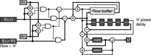
Gated filters are a related form of adaption to trimmed filters. These use one function of the pixel values within the window to select between two or more different filters to produce an output, as represented in Figure 8.22. The gating is determined independently for each output pixel. A simple example of a gated filter is to detect the gradient within the window and only apply smoothing perpendicular to the gradient. Such filters apply smoothing along an edge to reduce noise without significantly blurring the edge. Another example is to determine whether the window is within a uniform region away from an edge or is adjacent to an edge. If an edge is present, an edge enhancement filter may be used, otherwise a noise smoothing filter can be selected. At the extreme, a statistical test may be performed to determine if the pixel values come from a single Gaussian distribution (Gasteratos et al., 2006). If so, the mean can be used to smooth the noise, otherwise the original pixel value is retained to prevent degrading edges (which will generally have a mixed distribution).
Figure 8.22 Gated filter.
Nonlinear combinations of linear filters can also provide more useful outputs than a simple linear filter. Perhaps the most common example of this are the Prewitt and Sobel edge detection filters (Abdou and Pratt, 1979), which combine the outputs of two linear gradient filters; one in the horizontal direction and one in the vertical direction. Let H be the horizontal gradient and V be the vertical gradient. The magnitude of the two-dimensional gradient is ideally given by:
If the edge orientation is also required, this may be conveniently calculated using a CORDIC unit (Section 5.4.3) to calculate both the arctangent and Equation 8.16. However if just the edge strength is required, Equation 8.16 is quite expensive and two simpler alternatives are commonly used (Abdou and Pratt, 1979):
(8.17) ![]()
or
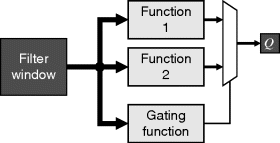
One example of a Sobel filter implementation is given by Hezel et al. (2002); it directly implements the two linear filters and combines the result. However, a simpler implementation may be devised that reduces the number of calculations by exploiting separability. Both the horizontal and vertical filters are separable and may be decomposed, as shown in Figure 8.23. The two filters are combined using Equation 8.18 to reduce the complexity.
Figure 8.23 Sobel filter implemented as parallel separable filters. Left: filter decomposition; right: implementation using Equation 8.18.

One limitation of differencing filters to detect gradients is that differentiating is a high pass operation and is, therefore, sensitive to noise. An alternative that has been proposed are moment-based filters (Suciu and Reeves, 1982), which are based on adding or integrating and are, therefore, inherently less sensitive to noise. The basic principle for edge detection is that the centre of gravity will be moved from the centre of the window in the presence of an edge. The offset of the centre of gravity from the window centre indicates the magnitude of the edge, while the direction is perpendicular to the edge orientation.
While there are many useful nonlinear filters, only a few of these are described in the following Sections.
8.3.1 Edge Orientation
The orientation of edges, or intensity gradients, within an image may be determined by taking the derivatives in two perpendicular directions. If necessary, the effects of noise may be reduced by applying a Gaussian or other noise smoothing filter before detecting the gradients. The two derivatives can then be treated as the components of the gradient vector. The orientation of the gradient may then be determined from the angle of the vector by taking an arctangent. This process is illustrated in Figure 8.24.
Figure 8.24 Edge orientation. The circle shows the mapping between angle and output pixel value.

In many situations, the output angle is required in terms of neighbouring pixels. Rather than perform the arctangent and then quantise the result, the orientation may be distinguished directly. Figure 8.25 shows some of the possibilities. To distinguish between a horizontal or vertical gradient, a threshold of 45° may be evaluated by comparing the magnitudes, as shown on the left. If necessary, the sign bits of the gradients may be used to distinguish between the four compass directions. The logic for this is most efficiently implemented using a lookup table to give the two bits out. If an eight-neighbourhood is required, the threshold angle is 22.5°. A sufficiently close approximation in most circumstances is:
Figure 8.25 Circuits for detecting limited orientations. Left: distinguishing horizontal and vertical; centre: four directions (0°, ±90°, 180°); right: including diagonal directions (0°, 45°, 90°, 135°, or 0°, ±45°, ±90°, ±135°, 180°).

(8.19) ![]()
which corresponds to a threshold of 26.6°. This will give a small preference to horizontal and vertical gradients over the diagonals. Again, the sign bits are able to resolve the particular direction and which quadrant the diagonals are in.
8.3.2 Non-maximal Suppression
The Canny edge detector (Canny, 1986) first smoothes the image, then detects the gradient, and suppresses points that are not a local maximum along the direction of the steepest gradient. Since the Gaussian smoothing will also spread the edge, the detector defines the position of the maximum gradient as the location of the edge. Non-maximal suppression is therefore thinning the edges, keeping only those points where the edge is the strongest.
Identifying the maximum gradient points first requires determining the orientation of the edge (from the direction of the steepest gradient). This may be determined as either horizontal or vertical or one of the two diagonals using the scheme described in the previous Section. If the gradient magnitude at a point is larger than both points on either side in the direction of the gradient, then the magnitude is kept. Otherwise, it is not a local maximum and reset to zero. One possible circuit for implementing this is in Figure 8.26. An alternative for determining both the magnitude and orientation is a CORDIC block, although only two bits are required for the orientation. The orientation must be delayed by one row to compensate for the latency of getting the magnitude on the row below the current pixel. The orientation is used to select the two adjacent magnitudes for comparison. If either of the neighbours is greater, this masks the output.
Figure 8.26 Non-maximal suppression for the Canny edge detector.

8.3.3 Zero-Crossing Detection
A zero-crossing detector is required to detect the edge locations from the output of Laplacian of Gaussian or difference of Gaussian filters. Whenever two adjacent pixels have opposite sign, it must cross through zero somewhere in the space between the two pixels (only very occasionally does the zero-crossing occur precisely at a pixel location). The pixel on the positive side of the edge is arbitrarily defined as being the location of the zero crossing. Referring to Figure 8.27, if the centre pixel is positive and any of the four adjacent pixels is negative, then the centre pixel is a zero-crossing. Just using the sign bit also handles the case when the centre pixel is exactly zero.
Figure 8.27 Zero-crossing detection filter. Left: definition of pixel locations within the window; centre: all zero crossings; right: those above a threshold.
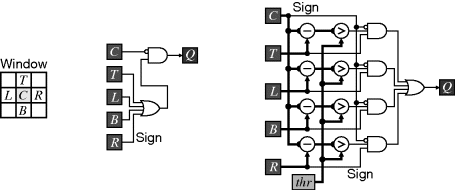
The zero-crossings will form closed contours within a two-dimensional image. However, many of the detected crossings will correspond to insignificant or unimportant features. A cleaner edge image may be obtained by requiring the adjacent pixels to not only be of opposite sign, but also be significantly different. This thresholding is shown in the right panel of Figure 8.27.
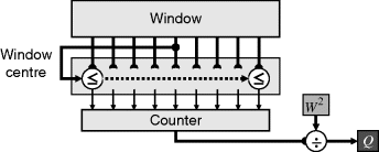
An important class of nonlinear filters is rank filters (Heygster, 1982; Hodgson et al., 1985). These rank the pixel values within the window and use the value from a selected rank in the list, as illustrated in Figure 8.28. They can be considered as a generalisation of the minimum, maximum (Nakagawa and Rosenfeld, 1978) and median filters. The main component of a rank filter is the sorting network that arranges the pixel values in ascending order. Obviously, if only a single, constant rank position is required, then only that sorted output needs to be produced by the sorting network, and the multiplexer is not required.
Figure 8.28 Rank filter.

Rank filters, or combinations of rank filters, can be used in a wide range of image processing operations.
Using ranks close to the median will discard outliers giving them good noise smoothing properties, especially for heavy tailed distributions. This is demonstrated in Figure 8.29 by almost completely removing the salt and pepper noise from a heavily corrupted image. In terms of additive Gaussian noise, the median is not as effective as an unweighted average of the same size. The best characteristics of both filters may be obtained by taking a weighted average of several ranks (Bovik et al., 1983).
Figure 8.29 Median filter. Top: salt and pepper noise with 12% pixels corrupted; bottom: additive Gaussian noise.
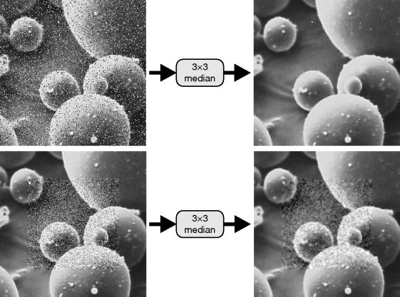
Straight edges are not affected by median filters, although if the edge is curved its position can shift, affecting the accuracy of any measurements made on the object (Davies, 1999). In the absence of noise, median filters do not blur edges (Nodes and Gallagher, 1982). However, any noise will cause edges to be slightly blurred, with the level of blurring dependent on the noise level (Justusson, 1981).
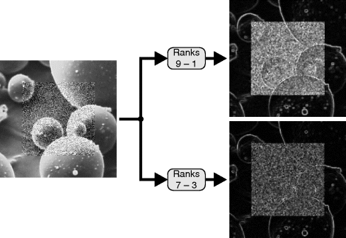
To detect edges, two rank values must be used and the difference between them is taken (Bailey and Hodgson, 1985), effectively using the range or subrange of pixel values within the window. The way this works as an edge detection filter is that each rank filter will shift the edges within the image by differing amounts, so the pixel difference will be larger in the vicinity of an edge. Generally a 3 × 3 window is used for edge detection; using a larger window will result in thick responses at the edges. The ranking of the pixels within the window means that the filter can detect edges of all orientations, and that the output of the filter is always positive. Using rank values closer to the extremes will give a stronger response, but is also more sensitive to noise. Rank values closer to the median are less noise sensitive, but will give a weaker response. These effects are clearly seen in Figure 8.30.
Figure 8.30 Subrange filters for edge detection.
A simple gated rank filter can be used for both enhancing edges while simultaneously suppressing noise (Bailey, 1990). Consider a blurred edge as shown on the left in Figure 8.31. When the centre of the window is over the edge, there are several pixels on either side of the edge. These will be selected by rank values near the extremes. Let the pixel values selected by the rank filters to be representative of the dark and light sides of the edge be D and L respectively. An edge enhancement filter classifies the centre pixel as being either light or dark depending on which is closer:
Figure 8.31 Rank-based edge enhancement filter. Left: pixels on either side of a blurred edge; right: edge enhancement using ranks 8 and 2.

Selecting the extreme values for D and L will be more sensitive to noise and outliers, and will tend to give a slight over enhancement. Ringing is completely avoided because one of the pixel values within the window is always selected for output. Selecting rank values closer to the median will give some edge enhancement, while at the same time filtering noise.
The rank-based edge enhancement filter is particularly effective immediately prior to multilevel thresholding and can almost completely eliminate the problems described in Section 6.1.2. It also makes threshold selection easier because the classification process of Equation 8.20 depopulates the spread between the histogram peaks that results from pixels that are a mixture of two regions. The thresholding results are therefore less sensitive to the exact threshold level used. For best enhancement, the size of the window should be twice the width of the blur. Then whenever the window is centred over a blurred edge, there will be representatives of each side of the edge within the window to be selected.
Since rank filtering involves sorting the pixel values within the window, any monotonically increasing transformation of the pixel values will not change the order of the pixel values. Rank filters are therefore commutative with monotonic transformations. Note that the results of rank-based edge detection or edge enhancement will be affected, because the output is a function of multiple selected values, and the relative differences will in general be affected by the transformation.
8.4.1 Rank Filter Sorting Networks
Key to the implementation of rank filters is the sorting network that takes the pixel values within the window and sorts them into ranked order. A wide range of techniques has been developed for implementing this, both in software and in hardware.
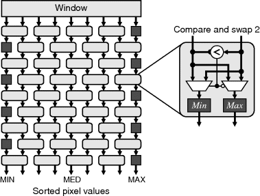
Perhaps the simplest and most obvious approach is to use a simple bubble sorting odd–even transposition network, as shown in Figure 8.32. To sort a whole window at the clock rate, it is necessary to pipeline each stage in the network. This simple approach is only really suitable for small windows because the amount of logic grows with the square of the window area.
Figure 8.32 Bubble sorting using an odd–even transposition network.
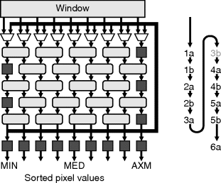
As with linear filters, running the filter with a higher clock rate (using a multiphase design) can reduce the hardware requirements. In this case it is complicated by the fact that the odd and even layers alternate. A two-phase scheme is shown in Figure 8.33. For sorting a 3 × 3 window, the number of layers has been reduced from nine to five. At the bottom, the data is looped back for a second pass through the network on the opposite phase. Note that since the bottom layer and the top layer are the same, phase 3b will not actually perform any sorting, but is required to phase shift the data fed back to interleave it with the new incoming data from the window.
Figure 8.33 Two-phase rank sorting network. Right: phasing of the data as it passes through the network.
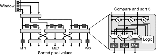
An improvement may be gained by exploiting the fact that there is considerable overlap between successive window positions. Significant savings may be gained by sorting a column once as the new pixel comes into the window and then merging the sorted columns (Chakrabarti and Wang, 1994; Waltz et al., 1998). One arrangement of this is shown in Figure 8.34. Note that for three inputs it is both faster and more efficient to perform the comparisons in parallel and use a single, larger multiplexer than it is to use a series of three two-input compare and swap blocks. In the middle layer of compare and sorts, since the inputs are successively delayed with each window position, the middle comparator can also be removed and replaced with the delayed output of the first comparator. This reduces the number of comparators from 36 required for a bubble sort to 14. Again, this can be further reduced if not every rank value is required.
Figure 8.34 Sorting columns first, followed by a merging.
A similar analysis may be performed for larger window sizes. Although savings can be gained by sorting the columns only once, the logic requirements still increase approximately with the square of the window size.
Rather than sort the actual pixel values, each pixel in the window can have a corresponding rank register which counts the number of other pixels in the window greater than that pixel (Swenson and Dimond, 1999). Then, as new pixels are added to the window, it is necessary to compare the incoming pixels with each of the existing window pixels to determine their rank and to adjust the ranks of the existing pixels. For one-dimensional filtering, a systolic array may be used to efficiently compare each pixel with every other pixel in the window and assign a rank value to each sample. One way of extending this to two dimensions is to collapse the two-dimensional window to one dimension by inserting the whole new column at each step (Hwang and Jong, 1990). The output is then taken every ![]() samples after the complete window has been processed.
samples after the complete window has been processed.
An alternative approach is to use the threshold decomposition property of rank filtering (Fitch et al., 1984; 1985). Rank filtering is commutative with thresholding, so if the image is thresholded first, a binary rank filter may be used. Therefore, a grey-level rank filter may be implemented by decomposing the input using every possible threshold, performing a binary rank filter, and then reconstructing the output by adding the results. This process is illustrated in Figure 8.35.
Figure 8.35 Threshold decomposition – the window values are thresholded to enable separate binary filters and reconstructed by combining the outputs.
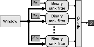
A simple implementation of a binary rank filter is to count the number of ones within the window and compare this with the rank value, as shown in Figure 8.36. The counter here is parallel; it is effectively an adder network, adding the inputs to give the count. As with other implementations, it is possible to exploit the significant window overlap for successive pixels. An implementation of this is shown on the right in Figure 8.36. The column counts are maintained, with the new column added and the old column subtracted as the window moves. This reduces the size of the counter from W2 to W inputs.
Figure 8.36 Binary rank filter for threshold decomposition. Left: thresholding to create binary values, and counting; right: an efficient implementation exploiting commonality between adjacent window positions.

Threshold decomposition requires ![]() parallel binary rank filters. This is expensive for small windows, but becomes more efficient for larger window sizes. This principle of threshold decomposition may also be generalised to stack filters (Wendt et al., 1986).
parallel binary rank filters. This is expensive for small windows, but becomes more efficient for larger window sizes. This principle of threshold decomposition may also be generalised to stack filters (Wendt et al., 1986).
A closer look at the left panel of Figure 8.36 reveals that the count produced is actually the bin from cumulative histogram of the window corresponding to the threshold, thr. An early software approach to median filtering was based on maintaining the running histogram of the window, updating it as the data moved into and out of the window (Garibotto and Lambarelli, 1979; Huang et al., 1979). There are two problems with directly using a histogram. The first is that for two-dimensional windows, multiple bins must be updated simultaneously, although this can be overcome by using a trick similar to that shown in the right panel of Figure 8.36. The second problem is that the histogram must be searched to find the corresponding rank value. The search may take many clock cycles to find the appropriate output value. These problems may be overcome by using the cumulative histogram. This approach was used by Fahmy et al., (2005) for one dimensional windows. An alternative to the direct output shown in Figure 8.35 is to use a binary search of the cumulative histogram (Harber and Neudeck, 1985). This is illustrated in Figure 8.37 for 3-bit data words. Note that in the right panel, the cumulative histogram counts are arranged in a bit-reversed order to minimise the interconnect length. The binary search can easily be extended to wider words, using pipelining if necessary to meet timing constraints. The binary search circuitry needs to be duplicated for each rank value required at the output.
Figure 8.37 Searching the cumulative histogram (illustrated for 3-bit data). Left: parallel approach of Figure 8.35; right: binary search.

This binary search can be extended to work from the original data using a bit voting approach. The idea is to reduce the logic by performing a binary sequence of threshold decompositions, with each decomposition yielding one bit of the output (Ataman et al., 1980; Danielsson, 1981). The threshold decomposition is trivial, selecting the most significant bit of those remaining, while passing on the remaining bits to the next stage. If the most significant bit of the input differs from the desired rank output, that input pixel value can never be selected for the rank output. This is achieved by setting the remaining bits to zero or one accordingly to prevent them from being selected in subsequent stages. The circuit for this scheme is shown in Figure 8.38. Note that only a single rank value is output; to produce additional rank values, the sorting network must be duplicated.
Figure 8.38 Bit sequential rank sorter.
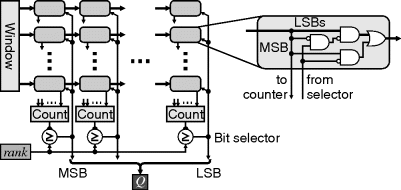
A scheme similar to this has been implemented on an FPGA by Benkrid et al. (2002a); Benkrid and Crookes (2003) for median filtering and by Choo and Verma (2008) for rank filtering.
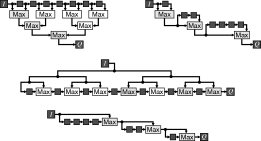
Minimum and maximum filters with rectangular windows are separable, providing an efficient implementation for large window sizes. A one-dimensional filter may be applied to either the rows or columns first, followed by a second one-dimensional filter in the other direction. The overlap in window positions as the window moves enables the filter to be efficiently implemented using ![]() operations (Bailey, 2010b). The basic principle is shown in Figure 8.39 for
operations (Bailey, 2010b). The basic principle is shown in Figure 8.39 for ![]() . To find the maximum requires
. To find the maximum requires ![]() two-input maximum operations. To minimise propagation delay, these may be arranged in a tree as shown in the top left panel. Since the inputs are sequential, the operations shown with a white background have already been calculated and can be buffered from before. The buffered version is shown in the top right panel. The circuit can readily be modified for window lengths that are not a power of two simply by reducing the number of delays in the last stage. The middle and bottom panels show a similar reuse transformation applied to the transposed filter structure (swapping input with output, and maximum operations with pick-off points). In the version which exploits reuse, the number of delays in the first stage can be reduced for window lengths that are not a power of two. Figure 8.39 illustrates a row filter; to implement a column filter, the sample delays are replaced by row buffers in the manner of Figure 8.18.
two-input maximum operations. To minimise propagation delay, these may be arranged in a tree as shown in the top left panel. Since the inputs are sequential, the operations shown with a white background have already been calculated and can be buffered from before. The buffered version is shown in the top right panel. The circuit can readily be modified for window lengths that are not a power of two simply by reducing the number of delays in the last stage. The middle and bottom panels show a similar reuse transformation applied to the transposed filter structure (swapping input with output, and maximum operations with pick-off points). In the version which exploits reuse, the number of delays in the first stage can be reduced for window lengths that are not a power of two. Figure 8.39 illustrates a row filter; to implement a column filter, the sample delays are replaced by row buffers in the manner of Figure 8.18.
Figure 8.39 Reducing the number of operations in a maximum filter. Top left: a tree structure requires ![]() operations; top right: exploiting reuse reduces this to
operations; top right: exploiting reuse reduces this to ![]() operations; middle: transposed tree structure, requires
operations; middle: transposed tree structure, requires ![]() operations; bottom: exploiting reuse in the transposed structure.
operations; bottom: exploiting reuse in the transposed structure.
While the median and other rank filters are not separable, a separable median can be defined that applies a one-dimensional median filter first to the rows then to the columns of the result, or vice versa (Shamos, 1978; Narendra, 1981). Although this is not the same as the true two-dimensional median, it is a sufficiently close approximation in most image processing applications. It also gives a significant savings in terms of computational resources. Note that in general a different result will be obtained when performing the row or column median first.
8.4.2 Adaptive Histogram Equalisation
Closely related to rank filtering is adaptive histogram equalisation for contrast enhancement. Global histogram equalisation, as described in Section 7.1.2, is ineffective if there is a wide variation in background level, making the global histogram approximately uniform. Adaptive histogram equalisation overcomes this problem by performing the transformation locally, attempting to make the pixel values within a local window be equally likely. This expands the contrast locally, while making the image more uniform globally.
Adaptive histogram equalisation is therefore a filter that determines the histogram equalisation mapping within a window, with only the centre pixel value being transformed. Each pixel is subject to a separate mapping based on local context (Hummel, 1977). Since each transformation is given by the scaled cumulative histogram within the window, the output is effectively the scaled rank position of central pixel value within the window (Pizer et al., 1987).
What makes adaptive histogram equalisation computationally expensive is that it generally uses a large window. To overcome this, many software implementations divide the image into a series of overlapping blocks and either use a single transformation for all of the pixels within each block or interpolate the transformations between blocks and apply the interpolated transformation to each pixel (Pizer et al., 1987).
Rather than build the histogram or cumulative histogram from scratch at each window position, it is possible to use an approach similar to that for box filtering to exploit adjacency and to update the histogram based on the changes. This approach was taken by Kokufuta and Maruyama (2009) and is represented in Figure 8.40. The basic approach is to maintain column histograms within the window. As the window moves to the next pixel, the histogram for the new column is updated and added to the window histogram. The column that has just left the window is subtracted from the window histogram. The column histograms must be cached in a row buffer until the next line. Since the histograms must be added and subtracted in parallel, they must be stored in registers, although a block RAM may be used for the histogram row buffer. Shallower fabric RAM or shift registers can be used to provide the W pixel delay unless W is large enough to make efficient use of a block RAM. The two delays in the window centre account for the latency of the histogram accumulation. The window histogram entries from bins less than the centre are summed to give the corresponding cumulative histogram bin, which is normalised to give the output pixel value.
Figure 8.40 Adaptive histogram equalisation by maintaining a running histogram.
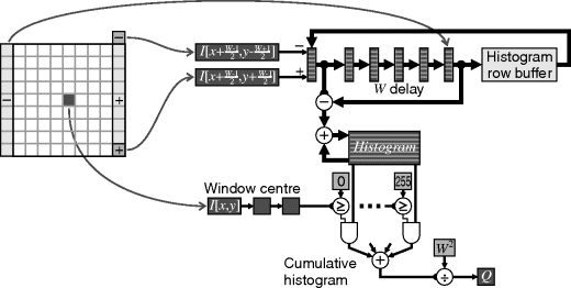
The resources required by this approach are independent of the window size. However, significant memory resources are required for the histogram row buffer and for registers for the column and window histograms. This approach is, therefore, suitable for large window sizes, although it does require a larger modern FPGA to provide the required on-chip memory.
For smaller window sizes, an alternative is to modify the threshold decomposition rank filter of Figure 8.36 to calculate the cumulative histogram bin for the current centre pixel value. This approach is demonstrated in Figure 8.41. Unfortunately, it is not possible to exploit the window overlap when moving from one pixel to the next because the threshold level varies with each pixel.
Figure 8.41 Adaptive histogram equalisation through window thresholding.
Filtering colour images carries its own set of problems. Linear filters may be applied independently to each component of the image.
Problems can be encountered when filtering hue images, because the hue wraps around. For example, the average of 12° and 352° is not 182° obtained by direct numerical averaging, but 2°. If the dominant hue is red (close to 0°), the hues may be offset by 180° before filtering and adjusted back again afterwards. The alternative is to convert from hue and saturation polar coordinates to rectangular coordinates before filtering and convert back to polar after filtering.
When using nonlinear filters, it is important to keep the colour components together. If a trimmed filter removes one component, all components should be trimmed. A gated filter should apply the same gating to all channels. Applying a nonlinear filter independently to each component can lead to colour fringing if the different components are treated differently.
Rank filtering, in particular, is not defined for colour images, because vectors do not have a natural ordering. This problem was discussed in more detail in Section 7.2.2. The median is, however, defined for colour data (Astola et al., 1988; 1990) and can be used for noise smoothing. One problem is the search through all of the points to find the median. For filtering, this must be performed within a pixel clock cycle. To do this efficiently, it is necessary to reuse the large proportion of data that is common from one window position to the next. Even so, efficient search algorithms, such as proposed by Barni (1997), are difficult to map to a hardware implementation. For small windows, the median may be calculated directly, although for larger windows the separable median may be more appropriate.
Many variations of the vector median filter have been proposed in the literature. The simplest is to interleave the bits from each of the components and perform a scalar median filter (Chanussot et al., 1999) with the wider data word. A wide range of gated vector medians has been proposed (Celebi and Aslandogan, 2008) that remove noise without losing too many fine details.
The rank-based edge enhancement filter can readily be adapted to colour images. The key is to identify when a pixel is on a blurred edge and then identify which of the two regions the edge pixel is most associated with. Consider three pixels across a boundary between two different coloured regions, as illustrated on the left in Figure 8.42. If point C is on a blurred edge between regions A and B, the colour will be a mixture of the colours of A and B:
Figure 8.42 Constructs for colour edge enhancement. Left: three pixels, with C on the border between regions A and B; centre: point C would be the vector median in the shaded region; right: a tighter criterion defined by Equation 8.25.

In this case, since C is between A and B, the central pixel C will be the vector median of the three points. In this case, from Equation 7.65:
(8.22) ![]()
or
If this is used as the criterion for detecting an edge pixel as proposed in (Tang et al., 1994), a point C anywhere in the shaded region in the centre panel of Figure 8.42 would be considered an edge pixel and enhanced. In three dimensions, this is a discus-shaped region, which can include points that deviate considerably from Equation 8.21. If C is indeed a mixture of the two colours, then:
(8.24) ![]()
An alternative edge criterion, allowing for some small deviation from the line as a result of noise, is (Gribbon et al., 2004):
which is an ellipsoidal region, illustrated by the shaded region in the right panel of Figure 8.42. T can either be fixed, or it may be proportional to the distance between A and B. In Figure 8.42, T is ![]() , which can easily be calculated using a simple shift.
, which can easily be calculated using a simple shift.
If C is an edge pixel, as determined by either Equation 8.23 or Equation 8.25, then the edge pixel may be enhanced by selecting the closest:
(8.26) ![]()
otherwise it is left unchanged.
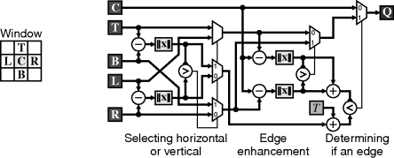
In extending to two dimensions, using a larger two-dimensional window presents a problem because of the difficulty in determining which two pixels in the window are the opposite sides of the edge (the A and B above). One alternative is to apply the one-dimensional enhancement filter to the rows and columns (Tang et al., 1994). An alternative is to check if the edge is primarily horizontal or vertical and perform the enhancement perpendicular to the edge (Gribbon et al., 2004). This approach is shown in Figure 8.43 using the edge detection criterion of Equation 8.25.
Figure 8.43 Colour edge enhancement.
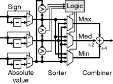
The distances may be measured using either the L1 or L2 norms. The L1 norm has the advantage that it is simple to calculate, although it is not isotropic. The L2 norm is isotropic, although for colours it requires three multiplications, two sums and a square root. The alternative is to use CORDIC arithmetic, although two CORDIC units are required for a three-component colour space. Since the norms do not need to be exact, an approximation to the L2 norm may be obtained by taking a linear combination of the ordered components (Barni et al., 2000). For three components, the relative weighting of the three components that gives the minimum error is (Barni et al., 2000) ![]() . A simple approximation that is reasonably close is 1 : 0.5 : 0.25, with the corresponding calculation represented in Figure 8.44.
. A simple approximation that is reasonably close is 1 : 0.5 : 0.25, with the corresponding calculation represented in Figure 8.44.
Figure 8.44 Simplified approximation of Euclidean distance (L2 norm).
If the edge blur is larger, then the same filter can be extended but considering points two or three pixels apart (Tang et al., 1994). If noise is an issue, the filter may be preceded by an appropriate noise smoothing filter (Tang et al., 1994).
For other operations, a common strategy is to apply the enhancement or filtering to the luminance component of the image (the Y from YUV or YCbCr, the V from HSV, or ![]() from L∗a∗b∗ or L∗u∗v∗). When doing so, it is important to keep the components together through any selection process to avoid colour fringing artefacts.
from L∗a∗b∗ or L∗u∗v∗). When doing so, it is important to keep the components together through any selection process to avoid colour fringing artefacts.
Based on set theory, mathematical morphology defines a set of transformations on a set based on a structuring element (Serra, 1986). In terms of image processing filters, the set can be defined by the pixel values within the image and the structuring element may be thought of as an arbitrary window. As implied by the name, morphological filters will filter an input image on the basis of the shape or morphology of objects within an image. The structuring element defines the shape of the filter and effectively defines or controls what is being filtered.
The basic principles of morphological filtering are easiest understood in terms of binary images. These principles can then be extended to filtering greyscale images.
8.6.1 Binary Morphology
A binary image considers each pixel to belong to one of two classes: object and background. In general the object pixels are represented by a binary 1 and the background is represented by 0. The structuring element, S, consists of a set of vectors or offsets. It can therefore be considered as another binary image or shape.
The basic operations of morphological filtering are erosion and dilation. With erosion, an object pixel is kept only if the structuring element fits completely within the object. Considering the structuring element as a window, the output is considered an object pixel only if all of the inputs are one; erosion is therefore a logical AND of the pixels within the window:
It is called an erosion, because the object size becomes smaller as a result of the processing.
With dilation, each input pixel is replaced by the shape of the structuring element within the output image. This is equivalent to outputting an object pixel if the flipped structuring element hits an object pixel in the input. In other words, the output is considered an object pixel if any of the inputs within the flipped window is a one, that is dilation is a logical OR of the flipped window pixels:
Note that the flipping of the window (rotation by 180° in two dimensions) will only affect asymmetric windows. In contrast with erosion, dilation causes the object to expand and the background to become smaller. Erosion and dilation are duals, in that a dilation of the image is equivalent to an erosion of the background and vice versa. This can also be seen in Equations 8.27 and 8.28 by taking the logical complement of both sides of the equation and using De Morgan's theorem.
Many other morphological operations may be defined in terms of erosion and dilation. Two of the most commonly used morphological filters are opening and closing. An opening is defined as an erosion followed by a dilation with the same structuring element.
(8.29) ![]()
The erosion will remove features smaller than the size of the structuring element and the dilation will restore the remaining objects back to their former size. Therefore, the remaining object points are only where the structuring element fits completely within the object.
The converse of this is a closing, which is a dilation followed by an erosion with the same structuring element.
(8.30) ![]()
Background regions are kept only if the structuring element completely fits within them. It is called a closing because any holes or gaps within the object smaller than the structuring element are closed as a result of the processing. Example morphological operations are illustrated in Figure 8.45.
Figure 8.45 Morphological filtering. In this example, black pixels are considered object, with a white background. (Photo courtesy of Robyn Bailey.)

The relatively simple processing and modest storage required by morphological filters has made them one of the most commonly implemented image processing filters, especially in the early days when FPGAs were quite small and the available resources limited what could be accomplished.
The direct implementation of erosion and dilation are relatively trivial, as seen in Figure 8.46. Duality enables both to be implemented with a single circuit, with a control signal used to complement the input and output.
Figure 8.46 Circuit for erosion and dilation. The control signal selects between erosion and dilation.
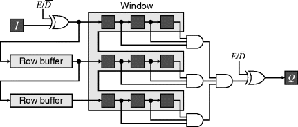
More interesting, however, is to make the structuring element programmable (Velten and Kummert, 2002). Associated with each window element is an additional register which controls whether or not that window element is part of the structuring element. It effectively gates the window data by providing a one from those window elements that are not part of the structuring element. The circuit of Figure 8.46 is modified to give Figure 8.47. The programme registers may be set either as part of the initialisation or programmed on-the-fly by another process.
Figure 8.47 Morphological filtering with a programmable structuring element.
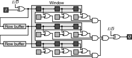
Opening and closing may be implemented as a pipeline of erosion followed by dilation, or dilation followed by erosion respectively. However, it is possible to combine both processes within a single window structure. Without loss of generality, consider the opening. By definition, if the complete structuring element fits within the object, all of those corresponding object pixels will be output. Therefore, by feeding back the erosion output, a parallel set of window registers may be used to hold the opening output. These must be shifted along because any of the window positions may set the output from the opening operation. This scheme is shown in Figure 8.48. Note that the row buffers have been changed to the serial configuration because the output must be shifted serially. The output multiplexer selects between erosion or dilation and opening or closing.
Figure 8.48 Extending the window operations to perform opening or closing as well as erosion or dilation using a programmable structuring element.
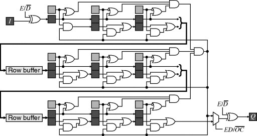
Although a single window structure is used, this filter has the same latency and row buffer memory requirements as a cascade of two filters. The advantage is that, for a programmable window, the structure element control bits are easier to share than if the two window filters were operated separately.
Just as linear filters could be decomposed as a sequence of simpler smaller filters, morphological filters can also be decomposed. There are two types of decomposition of particular interest here. The first is that dilation is associative, allowing a complex structuring element to be made up of a sequence of simpler structuring elements:
(8.31) ![]()
with a similar chain rule for a sequence of erosions:
(8.32) ![]()
The most obvious application of the chain rule is to make the operations for rectangular structuring elements separable, with independent filters in each of the horizontal and vertical directions.
The second decomposition is based on combining filters in parallel. For dilations:
(8.33) ![]()
and for erosions:
(8.34) ![]()
These decompositions, for example, allow the structuring element in Figure 8.45 to be decomposed as in Figure 8.49. Note that with decompositions, the integrated approach of performing the opening or closing demonstrated in Figure 8.48 cannot be used.
Figure 8.49 Example structuring element decompositions. Left: series decomposition using dilation; right: parallel decomposition using OR.

An alternative approach is to implement the filter directly as a finite state machine (Waltz, 1994c). Firstly, consider a one-dimensional erosion filter. The pattern of 1s and 0s in the window can be considered the state, as this information must be maintained to perform the filtering. If the structuring element is continuous, a useful representation of the state is the count of successive 1s within the window. The output is a 1 only when all of the inputs within the window are 1s. Therefore, whenever a 0 is encountered, the count is reset to zero, and when the count reaches the window width, it saturates. An example state transition diagram and corresponding implementation are given in Figure 8.50.
Figure 8.50 Horizontal erosion based on a state machine implementation. The shaded state outputs a 1, the other states output a 0. W is the size of the one-dimensional window.

This approach may be extended to arbitrary patterns by maintaining a more complex state machine. Basically the state is a compressed representation of the elements within the window. The finite state machine approach can also be extended to two dimensions by creating two state machines, one for operating on the rows and the other for operating on the columns (Waltz, 1994c; Waltz and Garnaoui, 1994a). It is not necessary for the structuring element to be separable in the normal sense of separability; the row state machine passes pattern information representing the current state of the row to the column state machine. This is illustrated for a non-separable structuring element in Figure 8.51.
Figure 8.51 Separable finite state machines for erosion with a non-separable window.
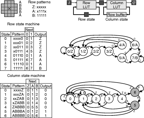
Firstly, the required patterns on each of the rows of the structuring element are identified. The row state machine is then designed to identify the row patterns in parallel as the data shifts in. Combinations of the row patterns are then encoded in the output to the column state machine. The column state machine then identifies the correct sequence of row patterns as each column shifts in. In this example, the row machine has only seven states and the column machine six states. The finite state machines may therefore be implemented using small lookup tables.
The technique may be extended to filters using several different structuring elements in parallel. The corresponding state machines are coded to detect all of the row patterns for all of the filters in parallel, and similarly detect the outputs corresponding to all of the different row pattern combinations in parallel.
The extension to dilation is trivial; the pattern is made up of 0s rather than 1s. It may also be extended to binary template matching (Waltz, 1994a), where the row patterns consist of a mixture of 0s and 1s (and don't cares). Binary correlation is implemented in a similar manner (Waltz, 1995), although it counts the number of pixels that match the template. The state machines for correlation are more complex because they must also account for mismatched patterns with appropriate scores.
8.6.2 Greyscale Morphology
Binary morphology requires that the image be thresholded before filtering. The concepts of binary morphology may be extended to greyscale images by using threshold decomposition. Reconstructing the greyscale image leads to selecting the minimum pixel value within the structuring element for erosion and the maximum pixel value for dilation. An alternative viewpoint is to treat the pixel value as a fuzzy representation between 0 and 1, and use fuzzy AND and OR in Equations 8.27 and 8.28 (Goetcherian, 1980). Either way, the resulting representations are:
and
with opening and closing defined as combinations of erosion and dilation as before.
Examples of greyscale morphological operations are illustrated in Figure 8.52. Opening removes lighter blobs from the image that are smaller than the structuring element, whereas closing removes darker blobs.
Figure 8.52 Greyscale morphological filtering.
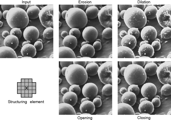
Any of the decompositions described for binary morphological filters also apply to their greyscale counterparts. The finite state machine implementation may also be extended to greyscale images (Waltz, 1994b), although significantly more state information is required to represent the greyscale pixel values. For rectangular structuring elements, efficient separable implementations as illustrated in Figure 8.39 are applicable.
For circular structuring elements, the structuring element may be decomposed using OR decomposition, with the corresponding rectangular windows implemented separably (Bailey, 2010b). Figure 8.53 demonstrates this for the 5 × 5 circular structuring element. The row buffers and delays are reused for both filters by merging the two filters. This requires that a transpose structure be used for the row filter. If necessary, additional pipeline registers may be added to reduce the delay through a chain of maximum operations, although on modern FPGAs the maximum processing rate is more likely to be limited by the timing for the row buffers.
Figure 8.53 Efficient circular window implementation. Top: OR decomposition of the structuring element; bottom: the separable implementation of both components. A transposed filter structure is used for the row filter. The numbers with the column filter represent the number of rows delay from the input. The numbers in the row filter represent the number of pixel delays to the output.

Equations 8.35 and 8.36 represent morphological filters with a binary structuring element. They may be further extended to use greyscale structuring elements:
(8.37) ![]()
and
(8.38) ![]()
The introduction of the extra component makes efficient implementation more difficult, because it is difficult to reuse results of previous calculations in all but special cases of the structuring element.
8.6.3 Colour Morphology
Extending morphological filters to colour images is more complex, because the equivalents of minimum and maximum do not exist for vectors. Simply applying the corresponding greyscale filters to each channel can give colour fringing where the relative contrast in different channels is reversed (for example on a border between red and green). The alternative (Comer and Delp, 1999) is to define a vector to scalar transformation that may be used for sorting the pixel values to enable a minimum or maximum pixel to be selected.
Adaptive thresholding is a form of nonlinear filter where the input is a greyscale image and output is binary, usually object and background. It is used when a single global threshold is unable to adequately separate the objects within the image from the background. There are two ways of looking at the operation. The first considers adaptive thresholding as a filter which calculates a suitable threshold based on the local context. The other is to consider the filter as a preprocessing step that adjusts the image enabling a global threshold be effective.
Since the goal of adaptive thresholding is to distinguish between object and background, the threshold level should be somewhere between the two distributions. The simplest estimate, therefore, is an average of the pixel values within the window, provided the window is larger than the object size. (A Gaussian filter gives a smoother threshold, although the unweighted box average is simpler to calculate.) This approach works best around the edges of the object, where thresholding is most critical, but for larger objects or empty background regions may result in misclassifications. These may be reduced by offsetting the average. This is illustrated in Figure 8.54 for the image of Figure 6.10 where global thresholding did not work. The delay in the main path is to account for the latency of the Gaussian filter.
Figure 8.54 Adaptive thresholding. Top: implementation; left: input image; centre: threshold level calculated using a Gaussian filter with ![]() and
and ![]() ; right: thresholded image.
; right: thresholded image.
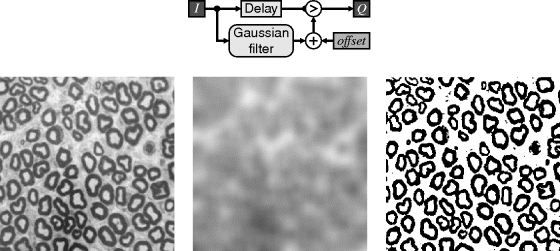
Another approach is to use morphological filtering to estimate the background level, which can then be subtracted from the image enabling a global threshold to be used. This approach is demonstrated in Figure 8.55.
Figure 8.55 Adaptive thresholding. Top: implementation; left: estimated background after using a morphological closing with a 19 × 19 circular structuring element to remove the objects; centre: after removing the background; right: thresholded image.
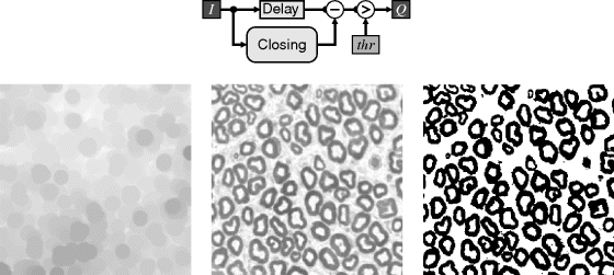
8.7.1 Error Diffusion
When producing images for human output, one problem of thresholding is a loss of detail. A similar problem occurs when quantising an image to a few grey levels, where the spatial correlation of the quantisation error results in contouring artefacts. What is desired is for the local average level to be maintained, while reducing the number of quantisation levels.
Floyd and Steinberg (1975) devised such an algorithm for displaying greyscale images on a binary display. The basic principle is that, after thresholding or quantisation, the quantisation error (the difference between the input and the output) is propagated on to the neighbouring four pixels that have not yet been processed. A possible implementation of this is shown in Figure 8.56. A row buffer holds the accumulated error for the next row, where it is added to the incoming pixel. The small integer multiplications can be implemented with a shift and add.
Figure 8.56 Binary error diffusion. (Photo courtesy of Robyn Bailey.)

The threshold is normally set at mid-grey. The thresholding is then equivalent to selecting the most significant bit of the input (and repeating it to give the equivalent output grey level as either black or white). The threshold level is actually arbitrary (Knuth, 1987); regardless of the threshold level, the errors will average out to zero, giving the desired average grey level on the output. Modulating the threshold level (making it dependent on the input) can be used to enhance edges (Eschbach and Knox, 1991), with the recommended level given as:
(8.39) ![]()
Although described here for a binary output, the same principles can be applied when any number of quantisation levels is used, by propagating the quantisation error to reduce contouring effects.
When applied to colour images, error diffusion may be applied to each component independently. With a binary output for each component, the outputs are in general uncorrelated between the channels. Threshold modulation may be used to either force correlation or anti-correlation between the channels (Bailey, 1997a). A simple modulation based on intensity (sum of RGB components) is sufficient to force resynchronisation. If the intensity is closer to black, the threshold level in all three channels can be increased by about 15% to encourage all three channels to simultaneously produce a 0 output. Similarly, if the intensity is closer to white, the threshold can be decreased to encourage all three channels to produce a 1. If the image is coloured, there will be a different number of 0s and 1s in each channel, but they will tend to cluster together as a result of the threshold modulation. To force anti-correlation, the opposite modulation can be used.
Local filters extend point operations by making the output depend not only in the corresponding input pixel value, but also its local context (a window into the input image surrounding the corresponding input pixel). To implement filters efficiently on an FPGA, it is necessary to cache the input values as they are loaded so that each pixel is only loaded once. The regular access pattern of filters enables the cache to be implemented with relatively simple row buffers, built from the block RAMs within the FPGA. When combined with pipelining of the filter function, such caching allows one pixel to be processed every clock cycle, making local filters ideal for stream processing.
Linear filters are arguably the most widely used class of local filters. The output of a linear filter is a linear combination of the input pixels within the window. Linearity enables such filters also to be considered in terms of their effect on different spatial frequencies; this aspect is explored more fully in Chapter 10.
One of the disadvantages of linear filters is their limited ability to distinguish between signals of interest and noise. A wide range of nonlinear filters has been developed to address this problem, of which only a small selection has been reviewed in this chapter. Two important classes of nonlinear filters considered in some detail are rank filters and morphological filters. A range of efficient structures for implementing these filters has been described in some detail.
Filtering colour images poses its own problems. Linear filters can be applied separately to each component, but for nonlinear filters it is important to treat the colour vector as a single entity. This is particularly so for rank and morphological filters, where edges within the image can be shifted as a result of filtering. To prevent colour artefacts, the edges within all components must be moved similarly.
Local filters are an essential part of any image processing application. Therefore, the range of techniques and principles described in this chapter is indispensible for accelerating any embedded image processing application.

