Chapter 6

The Equity Market

Gary L. Gastineau

ETF Consultants LLC

John F. Marshall

Marshall Management Services

Equity Market Snapshot

INTRODUCTION

This chapter examines some of the ways financial engineering has contributed, and will continue to contribute, to the growth of trading and the development of new products in the equity markets. The authors’ familiarity with U.S. markets is greater than their familiarity with other markets. Consequently, most of the examples are U.S. examples. This parochialism is not a significant disadvantage, because a similar story with similar examples is applicable to most of the world's equity markets.

CASH MARKET—ORIGINS

The cash equity markets exist to facilitate (1) the raising of equity capital by corporate issuers, and (2) the transfer of ownership interests in corporate entities among investors. The equity markets provide the essential mechanics and the necessary liquidity to accomplish these key objectives. Historically, the markets consisted of both centralized, highly organized, self-policing exchanges, and a less formal, over-the-counter component with markets made by dealers. In recent years a number of novel platforms have been introduced, including such things as “dark pools,” in which investors can trade anonymously. The roots of the modern equity markets in the United States trace back over 200 years, to the founding of what are now called the Philadelphia Stock Exchange and the New York Stock Exchange, respectively—both of which have undergone many transformations and mergers over the years.

The organization of equity markets varies from country to country, and, even within a country, there can be multiple market structures. Increasingly, mergers between exchanges, particularly cross-border mergers, have made the operation of equity markets a global enterprise. These mergers themselves can be seen as a form of financial engineering, as technologies developed and applied in one market are then transferred to another market. We will have more to say about the recent history of the cash equity markets later. But first we will consider some of the equity derivative products that have been developed and introduced over the past thirty or so years. These products represent milestones in the history of financial innovation. The more important of these are equity options, index options, stock index futures, equity swaps, and ETFs. Much of this chapter will be devoted to the latter.

EQUITY DERIVATIVES

There are a number of different types of equity derivatives, including equity options, exchange-traded index options, stock-index and single-stock futures, and equity swaps.

Equity Options

An equity option is routinely defined as the “right but not the obligation to buy or sell a specific number of shares of a specific stock at a specific price for a specific period of time.” The specific stock is called the “underlying asset” or simply the “underlying” (some people say “underlier”). The seller of the option is called the “writer,” the buyer of the option is called the “holder” or the “purchaser.” The seller is short the option, and the holder is long the option. For the “right” that the option conveys, the buyer of the option pays the seller of the option a “fee” up front, known as the “option premium.” The premium is the price paid for the option. It should not be confused with the strike price, which is a separate price paid if and only if the option is exercised. If the option gives its holder the right to buy the stock, it is known as a “call option,” or simply a “call.” If the option gives its holder the right to sell the stock, it is known as a “put option,” or simply a “put.” The specific price at which the option can be “exercised” is called the option's “strike price” (also sometimes known as the “exercise price”), and the life of the option is called its “time to expiration” or “time to expiry.” The actual date of expiration is called “expiration date” or “expiry.”

Options come in a variety of “types,” sometimes called “styles.” These include American-type, European-type, and Bermudan-type. American-type options can be exercised by the holder at any time from the moment they are written until the moment they expire. European-type, on the other hand, can only be exercised at the very end of their lives. Bermudan-type are in between American and European, in that they can be exercised at several distinct points in their lives, but are not continuously exercisable the way American-type options are.

Equity options have traded informally in an over-the-counter environment for a very long time, but it wasn't until the formation of the equity options exchanges that standardization and clearinghouses were introduced. The first of these to trade equity options in the United States was the Chicago Board Options Exchange (CBOE), which began trading calls in 1973 and soon after introduced puts. Other exchanges followed, and eventually there were a handful of exchanges trading, essentially, the same products but written on different underlyings. That is, each exchange had a monopoly on the “names” it traded, which made it possible for market makers to maintain rather wide bid-ask spreads. Eventually, under pressure from regulators and potential competitors, these monopolies gave way to competition and, not surprisingly, bid-ask spreads soon narrowed.

In the same year that exchange-traded equity options were introduced, two academics, Fischer Black and Myron Scholes (later to be considered two of the most important contributors to the field that eventually became known as financial engineering), published the first complete option pricing model. It is not that others had not tried to develop option pricing models, but none had completely succeeded. Black and Scholes demonstrated that, under a specific set of assumptions, the value of an equity option is a function of five variables. These are sometimes referred to as the option's “value drivers.” They are (1) the current spot price of the underlying stock, (2) the strike price of the option, (3) the time to option expiration, (4) the interest rate, and the (5) the volatility of the price of the underlying stock. In their model, Black and Scholes assumed away dividends.

The Black-Scholes model was soon improved upon by Robert Merton. Their collective work is now often referred to as the Black-Scholes-Merton option pricing model. These models were revolutionary theoretical and technological breakthroughs that were derived using principles of stochastic calculus. At the time, few people working in finance had the necessary quantitative skills to fully appreciate these models. Nevertheless, it was possible to develop “tables” to tell a trader what an option was worth under a given set of value drivers.

In time, a number of alternative approaches were developed to value equity options. These included finite difference methods, numerical models, and simulation models, among others. Each approach has its own strengths and its own weaknesses. For example, some models are easily adapted to fit a slightly different set of assumptions (such as if the stock pays dividends); others are not easily adapted. At the same time, the less flexible model might be computationally faster than more flexible models.

Over time, options were introduced on a variety of underlyings, in addition to equities. These included options on interest rates, options on commodities, options on futures, and so on. With each new type of underlying and each new set of contract specifications, new models needed to be developed. Because models employ assumptions and reality does not necessarily accord with the assumptions, new models are continuing to be introduced and old models refined. The goal is always to more accurately estimate the true value of the option. Indeed, option valuation modeling is one of the critical components of financial engineering expertise, and it is where you see the importance of a good quantitative skill set. It is also, in part, the reason that people associate financial engineering with quantitative finance—even though there are areas of financial engineering that do not require strong quantitative skills. Because this is not a chapter on derivatives valuation, we will only highlight the more elementary issues. We assume that the reader has access to more detailed literature on the mathematics of derivatives valuation.1

Today, equity options exchanges can trade options that are either physically deliverable or cash settled. Physically deliverable options require that, if the option is exercised, the physical underlying be transferred from one party to the other with payment simultaneously made at the contract's strike price. If the recipient of the underlying does not want the underlying, he or she can sell it in the cash market. Cash-settled options dispense with the physical transfer of the underlying and settle up at expiry for the cash equivalent of transferring the underlying and making a corresponding cash market transaction. For some purposes traders prefer physically deliverable options, but for other purposes cash settlement is more efficient.

Exchange-traded equity options employ a clearinghouse to remove the counterparty credit risk between the long and the short.2 That is, no matter with whom the actual trade is made when buying or selling the option, the trader's counterparty becomes the clearinghouse. The clearinghouse requires the option writer to post margin to protect the clearinghouse from credit risk. The buyer of the option pays the premium to the seller but does not post margin with the clearinghouse.

Even though not all options are cash-settled, and exchange-traded equity options are usually physically deliverable, we can talk about them as though they are all cash-settled since we can always synthesize cash settlement by a cash market transaction. We adopt this convention here.

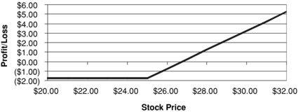
Exchange-traded equity options in the United States usually expire on the third Friday of the month. So, for example, a June call option on Microsoft (ticker MSFT) would expire on the third Friday of June. It is not necessary to point this out since all traders are familiar with this expiration convention. Now suppose that it is presently March 15 and the June option expires on June 19. That is 96 days to expiry. Suppose that MSFT is currently trading at $25.30 (the spot price), the relevant interest rate is 2 percent, and the annualized volatility of MSFT is 30 percent. Suppose further that MSFT will not pay any dividends between March 15 and June 19. We are interested in a call option having a strike price of $25. In this scenario, using a Black/Scholes’ set of assumptions, the value of this call is $1.76. Thus, ignoring a small bid-ask spread, the market maker would charge a $1.76 premium for this slightly “in-the-money” call option. The “per-share-covered” payoff to the option holder at expiry on June 19th would be given by the following equation:

where max denotes the “maximum” function defined as the larger of the two values in brackets at expiration, S denotes the spot price of the stock (i.e., stock price) at expiration, and X denotes the strike price. A call is described as “in-the-money” when S > X; “at-the-money” when S = X, and “out-of-the-money” when S < X. Since the strike price of $25 was set at the time the option was written and does not change, we can fill this in and get:

It should be plainly obvious that, at expiry, the option has zero value at any stock price at or below $25. The call will have a positive value (payoff) equal to the difference between S and X whenever S > X. Suppose, for example, that MSFT is trading at $32.10 at the time of the option's expiration. Then the payoff is given by:

Importantly, this terminal payoff should not be confused with “profit.” After all, the option holder paid the option writer $1.76 for the option when he or she bought it. Therefore, profit at expiration is given by:

In our specific example, the profit would be $5.34 (i.e., $7.10 – $1.76). Of course, this calculation is for each share covered by the option. On U.S. and most other countries’ exchanges, options typically cover 100 shares, so the actual premium paid and the actual profit earned on this contract would be $176 and $534, respectively.

Graphically, the profit diagram that corresponds to the profit/loss function above is depicted in Exhibit 6.1. Notice the characteristic “hockey stick” shape of the profit diagram. Whenever “hockey stick” shaped profit diagrams are encountered, one should always expect to find some sort of option.

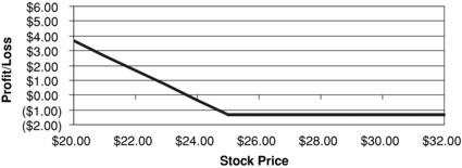
Analogous arguments can be made for put options. In these cases, the terminal payoff is given by:

And the profit function at expiration is given by:

Not surprisingly, a put option is in-the-money when S < X, at-the-money when S = X, and out-of-the-money when S > X.

Suppose now that the put has a strike price of $25, the stock price is again $25.30 at the time the option is written, the annual volatility is 30 percent, the interest rate is 2 percent, and the option has 96 days to expiry. The fair value of this slightly out-of-the-money put is $1.33, and we will assume that this is the price the buyer of the put pays. The profit function at expiry would then be given by:

And the profit diagram is given in Exhibit 6.2.

Exchange-Traded Index Options

Exchange-traded index options are options written on stock indexes, such as the S&P 500 or the NASDAQ 100. That is, the index is the underlying. They are typically cash settled at expiration rather than physically delivered. The key difference between equity options and index options is that the former are written on individual equities, while the latter are written on stock indexes. Pricing models for index options are similar to option pricing models for equity options. The terminal payoff function, the profit/loss function, and the profit diagrams for index calls and puts are identical to those for single-stock calls and puts.

Index options were introduced by the CBOE in 1983 under long-term licensing agreements from the publishers of the indexes (i.e., the trademark holders). This has given the CBOE a monopoly position in these contracts and has made it difficult for other exchanges to compete in these product areas. Similar index option products were introduced on European and Asian exchanges.

Stock-Index and Single-Stock Futures

In the United States, stock index futures contracts were introduced in 1982 by the Chicago Mercantile Exchange (CME). The CME, like the Chicago Board of Trade (CBOT),3 started out as a commodities exchange (also known as a commodity futures exchange). It wasn't until the 1980s that the CME began to introduce futures on underlyings that were not “commodities” in the traditional sense. The introduction of non-commodity futures, such as stock index futures and certain types of interest rate futures, required a “re-think” of the delivery rules for futures trading. The key innovation in the introduction of these two products, now some of the most heavily traded futures in the world, was the recognition that physical delivery could be replaced by cash settlement, provided that transparent cash settlement rules could be adopted.

It is important to note that index futures, like all futures, are guaranteed by a clearinghouse designated by the exchange. This effectively eliminates counterparty risk for the trading public. This is the same mechanism used to guarantee performance on exchange-traded equity options. However, in the case of futures, both parties to a futures contract post margin, which, in turn protects the clearinghouse from counterparty risk. Futures contracts are discussed much more thoroughly in the Commodity Market chapter of this book, so we will not spend precious space here describing the market mechanics of futures. Suffice it to say that stock index futures provided portfolio managers with a very useful hedging tool for their equity portfolios. They also provided investors with a highly-leveraged product that could be used to quickly and easily take either long or short positions on the broad market. Arbitrageurs, too, found uses for stock index futures, including various forms of basket trading that collectively became known as program trading.

As a side note, in 2002 a number of exchanges began trading single-stock futures (SSFs). These are similar in concept to commodity futures, in that each futures contract is written on one specific underlying stock, just as a commodity futures contract is written on one specific underlying commodity. The mechanics of SSFs, with respect to clearing and trading, are the same as the mechanics for index futures, and we won't elaborate on them here. The SSF market is small, but it has considerable future potential.

Equity Swaps

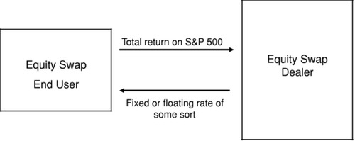
In 1989, Banker's Trust (later acquired by Deutsche Bank) introduced equity swaps. Equity swaps work on the same principle as interest rate swaps. These are over-the-counter derivatives and lack the standardization of most exchange-traded products. Indeed, that is one of their key strengths—they can be tailored to suit the specific needs of the client. In an equity swap, one counterparty pays the other counterparty a fixed or floating rate in exchange for receiving a floating rate determined by the behavior of a stock index (or a specific equity). The latter is paid on what is called the “equity leg.” The swap can make use of the “price return” of the stock or index, or it can make use of the “total return” of the stock, or index on the equity leg. Total return includes dividends, price return does not. A typical equity swap with a fixed or floating rate on the non-equity leg is depicted in Exhibit 6.3.

Equity swaps have many innovative uses, and the market for them grew rapidly after their introduction. The creation of this product was, of course, another exercise in financial engineering. So, too, was the introduction of each new variant of this product. Today there are dozens of such variants. The innovative applications of equity swaps are not to be neglected. These are best viewed as examples of applied financial engineering. We will consider one such example.

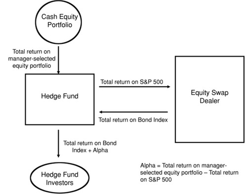
Suppose we have a hedge fund that seeks to earn the return on a bond portfolio. The hedge fund wants to “enhance” the return on the bond portfolio with some “alpha” earned from its expertise in the stock market. That is to say, the hedge fund manager believes he or she has the ability to outperform some equity benchmark (let's make it the S&P 500) on a risk-adjusted basis. So, the hedge fund purchases a carefully selected portfolio of equities. It then enters into an equity swap with an equity swap dealer. This equity swap is tailored a bit so that the hedge fund pays the dealer the total return on the S&P 500 quarterly for two years. In return, the equity swap dealer pays the hedge fund the total return on a particular bond index. Notice that this is the total return on an equity index for the total return on a bond index.

The logic here is that the hedge fund earns for its investors the total return on the bond index, just as if it had invested in the bonds that make up the index. But, it also keeps the difference between what it earned on its cash equity portfolio and what it pays on the equity leg of the swap. Assuming that the systematic risk of the equity portfolio and the systematic risk of the index used for the equity leg of the swap are the same, any difference could be a manifestation of “alpha.” This alpha can then be paid out with the bond index return to the investors in the fund. This is an example of using equity swaps to “port” alpha from one asset class (equities) to another asset class (bonds). Portable alpha is discussed later in this book in more detail. The structure is depicted in Exhibit 6.4.

Equity swaps have become particularly popular in Europe as a vehicle to avoid taxes on equity transactions. For example, the U.K. government levies a 0.5 percent “stamp duty” (the term comes from the old practice of requiring stamped paper for legal documents) on the purchase side of an equity transaction. By structuring an equity swap to synthesize a long or short position in equities, the investor does not have to pay this tax. Equity swaps of this sort are commonly called “contracts for difference” (CFD). CFDs are typically contracts between investors and dealer banks. At the end of the contract, the parties exchange the difference between the starting and ending prices of the underlying financial instrument. As a side point, investors in these sorts of equity swaps can also benefit by avoiding custody fees, withholding taxes on dividends, and restrictions on shorting stock. Recent estimates place CFD-backed trades at the equivalent of 25 percent to 30 percent of equity transactions on the London Stock Exchange.

The same OTC derivatives dealers that make markets in equity swaps also, often, make markets in equity options. These differ from exchange-traded equity options in that all terms are negotiable. Additionally, it is possible to create extraordinarily “exotic” equity swaps and equity options, which have many uses. These exotic products tend to be introduced when a client has a problem that none of the existing products neatly addresses. Once a novel product is introduced, it is often added to the dealer's toolkit and recycled to other clients. Through this process, the tailored exotic gradually becomes another off-the-shelf tool.

DECLINING TRADING COSTS INCREASE FINANCIAL ENGINEERING OPPORTUNITIES, AND FINANCIAL ENGINEERING OFTEN REDUCES TRADING COSTS

In 1968, the average daily volume of stock trading on the New York Stock Exchange (NYSE) was about 13 million shares. Just 40 years later, in 2008, the average daily trading volume in NYSE-listed stocks was about six billion shares per day. This is roughly a 450 times increase in volume, yet it still understates the significance of the increase in equity trading volume. In 1968, the trading volume on other exchanges and the over-the-counter market (not yet NASDAQ) was a small fraction of the trading volume on the New York Stock Exchange, and ETFs did not exist. In 2009, total equity trading volume was nearly 10 billion shares a day and about 20 percent of that volume was in ETFs.

New York Stock Exchange trading volumes in 1968 were at record levels—up from just three million shares a day in 1960. In fact, one reason for selecting 1968 as a starting point for this commentary is that this high volume (by the standards of the day) created massive operating problems for U.S. securities markets. The NYSE closed early on many days in the first half of 1968 and closed every Wednesday during the second half of the year to deal with a “paperwork crisis.”

The dramatic growth in trading over the next 40 years—without a repeat of the operational chaos of 1968—is the result of two kinds of changes that are at the heart of many examples of financial engineering: improvements in technology and corresponding changes in the economics of trading and in the instruments available to trade. The computerization of both trading and back office operations has sharply reduced commissions and trading spreads for small trades and for trading baskets of securities since 1968. The costs of large trades in a single issue have not, on the other hand, declined much, if at all, because their largest cost element is the price of the liquidity they demand.

Long before 1968 and for a few years thereafter, New York Stock Exchange commissions were fixed at a high level. The average commission on a stock purchase or sale in 1968 was significantly more than 1 percent of the value of the transaction. Bid-ask spreads were generally measured in quarters ($0.25) rather than the penny ($0.01) spreads common for small trades in many actively traded shares today. The market impact of a large trade was significant in 1968, as it is today. The growth of institutional investing was just getting under way in 1968, so large trades were much less common than they became in the 1970s and 1980s.

Punch-card accounting was still common in 1968, but the early computer systems available then were dramatic innovations relative to the handwritten ledgers and clerks with iconic eyeshades that were the state of the art 40 years earlier in the late 1920s. The technology introduced since the paperwork crisis of 1968 has made much higher volumes possible with far less hands-on human involvement in every step of the trading and trade settlement process.

The workday population on the New York Stock Exchange floor grew for a number of years after 1968, but floor trading activity is not meaningful today. Most recent live videos from the NYSE floor show more quotation monitors than people to watch them. The visitors gallery has been closed since September 11, 2001 and the floor is often most crowded during the cocktail parties that begin shortly after the formal close of trading. Automated trading and trade processing have changed the visualization, as well as the economics, of trading.

The total cost to buy or sell stock in 1968 approached 2 percent of the value of the stock. With some fairly rough rounding, total trading costs probably represented a little more than 0.2 percent of the value of the trade for the average transaction by a retail investor in 2008. The average cost of a typical retail transaction fell by a factor of nearly 10 while total transaction costs in the stock market increased by a multiple of as much as 50. The reduction in the cost of each trade brought in more traders—and facilitated a number of feats of financial engineering. While the increases in trading volume and in total trading costs are dramatic, they are an almost inevitable consequence of changes in technology and market infrastructure that stimulated a broad range of financial market innovations.

In some respects, the most dramatic equity trading stories are the stories of new equity derivatives markets and new derivative products that have been introduced on equity markets over the past 40 years. Many of these markets and products were briefly discussed in the first part of this chapter. These new equity derivatives markets have their own eye-popping figures for transaction volumes and the notional values of both trading and open interest in equity derivatives contracts. While new equity derivatives have stimulated stock volume, the notional volume in some of these equity derivatives markets exceeds the dollar value of the underlying equity market volumes.

As noted earlier, exchange-traded equity derivatives, such as index futures, single-stock futures, and equity options, all employ a clearinghouse to guarantee performance and ameliorate counterparty credit risk. OTC products, such as equity swaps, equity forwards, and OTC equity options have not, generally, employed a clearinghouse to guarantee performance. Instead, each participant in these bilateral transactions needed to consider the creditworthiness of its counterparty. This, of course, tended to push the end users of these contracts toward more highly rated dealers. Banks often responded by setting up “best credit” subsidiaries to serve as the dealer function. These would typically be very well-funded and have an excellent credit rating. However, in the wake of the credit issues that surfaced in 2007 and 2008, many of these OTC instruments will be cleared through clearinghouses in the future.

ARBITRAGE COMPLEXES

The relationships between trading in equities and trading in various equity derivatives markets are best understood by considering how an arbitrage complex works. The arbitrage complex provides a useful way to think about the range of choices open to users of index (or portfolio basket) financial instruments. The arbitrage complex consists of a number of related financial instruments, or groups of financial instruments, based on a common group of underlying assets. The principal underlying assets behind each of the instruments in an arbitrage complex may consist of an index, an arbitrary stock basket, an exchange-traded fund (ETF), or even an individual security or commodity. The arbitrage complex can cover domestic and/or foreign markets. An arbitrage complex can include components that are nominally debt instruments (structured notes), and it can include options and other components that have a nonsymmetric response to changing prices.

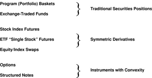
Exhibit 6.5 lists some typical equity index arbitrage complex instruments. Among the traditional securities positions, the members of the equity index arbitrage complex are program or portfolio trading of baskets of equity securities and exchange-traded funds. These are simply combinations and extensions of the traditional underlying securities that compose equity portfolios. Trading securities in a basket or as an index derivative is a natural extension of both trading technology improvements and modern portfolio theory.

The second category in the arbitrage complex is symmetric derivatives. By symmetric, we mean that they move up and down very much like the underlying index portfolio or position that determines their market risk characteristics. The most important symmetric equity index instruments are stock index futures, ETF single-stock futures contracts, and equity index swaps.

To round out the instruments that make up an equity index arbitrage complex, there are index options and structured notes based on indexes. In contrast to the instruments we have discussed so far, instruments with embedded options have convexity; that is, they have payoffs that are not straight-line functions of an underlying price variable.

We plan to spend most of the balance of this chapter illustrating and analyzing some of the things financial engineers have done and continue to do to transform key segments of the market in equity securities. The development of these markets illustrates some of the ways in which trading in the components of an arbitrage complex interact and contribute to pricing efficiency and trading cost reduction.

EQUITY STRUCTURED PRODUCTS AND EXCHANGE-TRADED FUNDS (ETFS)

The equity structured products that financial engineers have developed over the years are extraordinarily diverse. These structured products have ranged from structured notes (debt instruments with embedded equity elements) and covered warrants to Americus Trust primes and scores, which were similar to a number of products now available on the listed options markets. The most successful of the equity instruments developed by financial engineers go under the broad label of exchange-traded funds (ETFs). Not all the products called ETFs are funds, but most of them share a common genesis in basket or portfolio trading and index arbitrage. A few of them are simply different ways to package something—gold, for example—to make it easier for investors to hold and trade as a security. They are all exchange-traded. The fact that investors can trade most of the products called ETFs at market-determined prices that are close to the intraday value of an underlying portfolio or index is one common feature of most of these securities. At various times, the ETF label has been attached to:

• Closed-end funds (e.g., Nuveen).
• Grantor trust products based on fixed portfolios (e.g., HOLDRs).
• Grantor trust products based on holdings of a single commodity (e.g., Gold and Silver Trusts).
• Currency money market trusts (e.g., Euro Currency Trust).
• Commodity indexed trusts (e.g., iShares Goldman Sachs Commodity Index Trust).
• Open-end structured notes (e.g., iPath GSCI Total Return Index Notes).
• Mutual fund exchange-traded share classes (e.g.,Vanguard ETFs).
• Standard & Poor's depositary receipt (SPDR)-style indexed portfolios (e.g., SPDRs, QQQs, World Equity Benchmark Shares [WEBS], iShares, etc.).

Each of these products has an interesting history, and most can serve as models for further financial engineering. For reasons of space, our focus will be on the last group. It includes the largest number of products and competes head-to-head with conventional mutual funds, a product family in serious need of some structural innovation. As we look at ETF evolution we will take quick looks at where a few of the other products fit into the history of equity market innovation.

When we examine these products, it is important to bear in mind that many of the early ETFs were not created to provide a superior investment vehicle. Some of the most successful of these products were developed primarily to provide something to trade, not to create the ideal product for investors. Most of the products that are called ETFs rely heavily on a low-cost equity trading environment. Because of diverse motives and structural choices, it is often difficult to pin down the economic incentives to various parties behind a particular product or structure. Nonetheless, an important part of the financial engineer's job is to understand the economic incentives that will make a new product or market succeed. Cost reduction is usually a large part of the explanation for the success of a new product or market. Keep an eye out for examples of cost reduction as we trace the history of the ETFs’ antecedents—the proto-products that led to the current generation of ETFs—and set the stage for products yet to come.

PORTFOLIO TRADING AND STOCK INDEX FUTURES CONTRACTS

The basic idea of trading an entire portfolio in a single transaction did not originate with the Canadian Toronto Index Participation Securities (TIPs) or the U.S. SPDRs, the earliest examples of the modern portfolio-traded-as-a-share structure. It originated with what has come to be known as portfolio trading or program trading. From the late 1970s through the 1980s, program trading was the then-revolutionary ability to trade an entire portfolio, often a portfolio consisting of all the S&P 500 stocks, with a single order placed at a major brokerage firm. Similar portfolio trades were available using other indexes in Canada, Europe, and Asia. Some relatively modest advances in electronic trade entry and execution technology, and the availability of large order desks at some major investment banking firms, made these early portfolio or program trades possible. The introduction of S&P 500 index futures contracts by the Chicago Mercantile Exchange (and similar contracts in other markets) created and required an arbitrage link between the new futures contracts and portfolios of stocks. It was even possible, in a trade called an exchange of futures for physicals (EFP), to exchange a stock portfolio position, long or short, for a stock index futures position, long or short. The effect of these developments was to make portfolio trading either in cash or in futures markets an attractive activity for many trading desks and for many institutional investors. The attraction was a combination of opportunities for arbitrage profits and lower trading costs. The equity arbitrage complex is a natural consequence of these developments.

From developments that originally served only large investors, there arose interest in a readily tradable portfolio or basket product for small institutions and for individual investors. The early futures contracts were relatively large in notional size, and the variation margin requirements for carrying these futures contracts were cumbersome and relatively expensive for a small investor. The need for a low-price-point security (i.e., an SEC-regulated portfolio product) that could be used by individual investors was increasingly apparent. The first such products in the United States were index participation shares (IPS).

Index Participation Shares (IPS)

Index participation shares were a relatively simple, totally synthetic proxy for the S&P 500 index. While other indexes were also available, S&P 500 IPS began trading on the American Stock Exchange (Amex) and the Philadelphia Stock Exchange in 1989. A federal court in Chicago quickly ruled that the IPS were futures contracts and had to be traded on a futures exchange, if they were to be traded at all. The stock exchanges had to close down IPS trading. This would not have been an issue in most other countries. Outside the United States, securities and futures are typically overseen by the same regulator, and there is less legal distinction between a security and a futures contract.

While a number of efforts to find a replacement product for IPS that would pass muster as a security were underway in the United States, Toronto Index Participation Securities (TIPs) were introduced in Canada.

Toronto Index Participation Securities (TIPs)

TIPs were a warehouse receipt-based instrument designed to track the TSE-35 index and, later, the TSE-100 index as well. TIPs traded actively and attracted substantial investment from Canadians and from international indexing investors. The ability of the trustee to lend out the stocks in the TIPs portfolios for a fee led to a negative expense ratio at times. However, the TIPs proved costly for the Toronto Stock Exchange and for some of its members who, because of the simple (noncommercial) TIPs structure, were unable to recover their costs from investors. Early in 2000, the Toronto Stock Exchange decided to get out of the portfolio share business, and TIPs positions were liquidated or, at the option of the TIPs holder, rolled into a fund now known as the iShares CDN LargeCap 60. This fund had assets of about C$12 billion at the end of 2009.

Meanwhile, two other portfolio-in-a-share products were under development in the United States: SuperTrust and SPDRs.

SuperTrust and Supershares

The SuperTrust and Supershares were a product complex using both a trust and a mutual fund structure—one inside the other. Supershares were a high-cost product. The complexity of the product, which permitted division of the Supershares into a variety of components, some with option and option-like characteristics, made sales presentations long and confusing for many customers. The Supershares were developed by Leland, O’Brien, Rubinstein Associates, the folks behind portfolio insurance. The SuperTrust securities never traded actively, and the trust was eventually liquidated. This product failure stemmed from higher costs and greater complexity than investors were prepared for in the early 1990s. The failure was unrelated to portfolio insurance.

Standard & Poor's Depositary Receipts (SPDRs)

Standard & Poor's depositary receipts (SPDRs, pronounced “spiders”) were developed as a trading vehicle by the American Stock Exchange, approximately in parallel with the SuperTrust. The original SPDRs are a unit trust with an S&P 500 portfolio that, unlike the portfolios of most U.S. unit trusts, can be changed as the index composition changes. The reason for using the unit trust structure was the Amex's concern for costs. A mutual fund must pay the costs of a board of directors, even if the fund is very small. The Amex was uncertain of the demand for SPDRs and did not want to build a more costly infrastructure than was necessary. Only a few other ETFs (e.g., the MidCap SPDRs, the NASDAQ-100 QQQs, and the DIAMONDS, based on the Dow Jones Industrial Average) use the unit trust structure. Most ETFs introduced since 2000 use a modified version of the mutual fund investment company structure. Nonetheless, the S&P 500 SPDRs remain the largest ETF and the largest consumer equity investment product in the United States and the world, with assets of nearly $85 billion at the end of 2009.

SPDRs traded reasonably well on the Amex in their early years, but only in the late 1990s did SPDRs’ trading volume and asset growth take off, as investors began to look past the somewhat esoteric in-kind share creation and redemption process, and focus on the investment characteristics and tax efficiency of the SPDRs themselves. It is difficult to ascribe the phenomenal success of the SPDR and subsequent ETFs to a small list of factors, but certainly among the contributing features to the SPDRs’ success were: (1) extremely tight and aggressive market making by the specialist team at Spear, Leeds & Kellogg; (2) the fact that the Amex was able to get the SPDRs’ expense ratio below the expense ratio of the Vanguard 500 mutual fund, the SPDRs’ principal competitor; and (3) the steady growth of interest in the tax efficiency of exchange-traded funds, which usually permits the holder of this type of ETF to defer all capital gains taxation until the shares are sold. Note that these features all reflect the importance of cost reduction in the success of a new product.

World Equity Benchmark Shares (WEBS, Renamed iShares MSCI Series) and Other Investment Company Shares

The World Equity Benchmark Shares (WEBS) are important for two reasons. First, they are foreign index exchange-traded funds—that is, funds holding stocks issued by non-U.S.–based firms. Second, they are some of the earliest exchange-traded fund products to use a management investment company (mutual fund) structure as opposed to a unit trust structure. If you are going to create a large number of similar products, a mutual fund series structure can be much less costly to maintain than a separate unit trust for each product.

Another family of foreign index funds designed to compete with the WEBS was introduced on the NYSE at about the same time that WEBS appeared on the Amex. For a variety of reasons, the most important of which were structural flaws in the product, these country baskets failed, and the trust was liquidated.

The sector SPDRs were the first ETFs with domestic stock portfolios in a mutual fund structure similar to the WEBS. They were introduced in late 1998, and their assets have grown more consistently than most other specialized ETFs.

Other brands for ETFs and similarly traded products have included:

• Ameristock
• BLDRS (Baskets of Listed Depositary Receipts)
• Claymore
• Fidelity
• First Trust
• FocusShares
• HealthShares
• HOLDRS (Holding Company Depositary Receipts)
• MacroShares
• PowerShares
• ProShares
• Realty Funds
• Rydex
• SPA ETF Europe Ltd.
• State Street SPDRs
• StreetTracks
• TDAX Independence Funds
• VanEck
• Vanguard
• Victoria Bay
• Wisdom Tree

with new brands added frequently. Many of the same brands are represented in ETF markets outside the United States, and, of course, some firms offer funds in just one country or a small number of countries. At the end of 2009, there were more than 1,907 ETFs trading on 39 exchanges around the world with total assets of USD 1 trillion (Fuhr, 2009).

ETFs Not Operating under the Investment Company Act of 1940

The unit trust structure of the SPDRs, and the managed investment company structure of the WEBS, sector SPDRs, and other true funds launched after 2000 in the United States, are subject to the Investment Company Act of 1940, the legislation that covers the operation of mutual funds. In addition to these true funds, there are a number of other products under a broader definition of an ETF that are organized as a grantor trust, as another type of trust, or as an open-end exchange-traded note. These products exist because some portfolio products cannot be issued under the Investment Company Act of 1940. The Investment Company Act and related tax statutes restrict the type of financial instruments that can be held by an investment company and the type of income it can receive. As is their wont, financial engineers have developed a wide range of products that mesh with the securities laws in appropriate ways to package portfolios of securities, commodities, and derivatives for delivery in a convenient package that is not encumbered by some of the restrictions imposed by the Investment Company Act. Some of these are grantor trusts with pass-through of the incidents of ownership to the holders of shares in the trust. Others are in the form of limited partnerships, necessitating the distribution of K-1 tax reports to each investor in the United States.

Still others are relatively simple exchange-traded notes, which are open-ended to provide for expansion and contraction in a manner similar to the creation and redemption mechanism of the investment company ETFs. ETFs, in the broadest sense, have been an arena for significant financial engineering innovation, and there is no reason to expect the pace of innovation to decline. Nevertheless, one cannot help speculating that some of the low-hanging financial engineering fruit has been plucked and that the most fruitful area for innovation going forward will involve modifying the structure and operation of open-end portfolio ETFs.

Open-End Portfolio ETFs Subject to the Investment Company Act of 1940

The open-end ETFs based on the SPDR model (both unit trust and mutual fund structures) have a number of fundamental characteristics that have made this new generation of funds a worthy model for further development by financial engineers. These open-end ETFs do not have shareholder accounting expenses at the fund level, and they have few, if any, embedded marketing expenses. In a sense, they are like mutual funds stripped of some costly historical baggage. These expense-reducing features, and the fact that these fund shares are traded like stocks rather than like mutual fund shares, usually make ETFs more costly than no-load mutual funds to buy and sell, but nearly always less costly to hold than comparable mutual funds. Some early investors in ETFs were attracted by the fact that the ETFs were low-cost index funds. However, today's index funds—ETFs and mutual funds—are not always the low-cost portfolios their owners thought they were buying.

From a financial engineering perspective, it is useful to focus on two important characteristics of the SPDR-style ETF that were, in some respects, serendipitous. Because these characteristics have helped attract investors, they have been important in the early success of ETFs. These characteristics also provide a basis for development of the SPDR-style ETF model well beyond its impressive beginnings. Not everyone attaches as much significance as we do to these two features, but we are convinced that they hold the key to the development of better funds. The two key features of most existing SPDR-style ETFs are shareholder protection and tax efficiency.

SHAREHOLDER PROTECTION

The material described in the next few paragraphs is widely known, but not frequently discussed. A recent comprehensive description of mutual fund pricing over the years is available in Swenson (2005).4

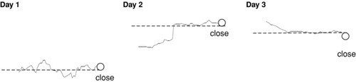
In 1968 (that year again), the Securities and Exchange Commission (SEC) implemented Rule 22(c)(1), which required mutual fund share transactions to be priced at the net asset value5 (NAV) next determined by the fund. This meant that anyone entering an order after the close of business on day 1 would purchase or sell fund shares at the net asset value determined at the close on day 2. Correspondingly, someone entering an order to purchase or sell shares after the close on day 2 would be accommodated at the net asset value determined at the close on day 3. This process is illustrated in Exhibit 6.6.

There is a transaction fairness problem for fund investors with Rule 22(c)(1) in place.6 That problem is illustrated in Exhibit 6.7.

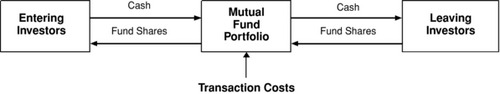
By pricing all transactions in the mutual fund's shares at the net asset value next determined, as required by Rule 22(c)(1), the fund provides free liquidity to investors entering and leaving the fund. All the shareholders in the fund pay the cost of providing this liquidity. As Exhibit 6.7 illustrates, anyone purchasing mutual fund shares for cash gets a share of the securities positions already held by the fund and priced at net asset value. The new investor typically pays no transaction costs at the time of the share purchase. All the shareholders of the fund share the transaction costs associated with investing the new investor's cash in portfolio securities. Similarly, when an investor departs the mutual fund, that investor receives cash equal to the net asset value of the shares when the NAV is next calculated. All the shareholders in the fund bear the cost of selling portfolio securities to provide this liquidity. To the entering or leaving shareholder, liquidity is essentially free. To the ongoing shareholders of the fund, the liquidity given to transacting shareholders is costly. Over time, the cost of providing this free liquidity to entering and leaving shareholders is a perennial drag on a mutual fund's performance.

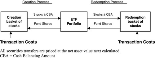
Exhibit 6.8 shows that exchange-traded funds handle the costs of accommodating entering and leaving shareholders differently from mutual funds. For exchange-traded funds, creations and redemptions of shares are typically made in-kind. Baskets of portfolio securities are deposited with the fund in exchange for fund shares in a creation. In a redemption, fund shares are turned in to the fund in exchange for a basket of portfolio securities. The creating or redeeming investor—often a market maker in the ETF shares—is responsible for the costs of investing in the portfolio securities for deposit, and the cost of disposing of portfolio securities received in the redemption of outstanding fund shares. The market makers even pay a modest creation or redemption fee to cover the fund's administrative expenses. The market maker expects to pass these transaction costs on to investors when the market maker trades fund shares on the exchange. The cost of entering and leaving a fund varies, depending on the level of fund share trading activity and the nature of the securities in the fund's portfolio. For example, the cost of trading in small-cap stocks can be much greater than the cost of trading in large-cap stocks.

SPDR-type ETFs are different from mutual funds in the way they accommodate shareholder entry and exit in at least two important ways. (1) As illustrated, the trading costs associated with ETF shareholder entries and exits are ultimately borne by the entering and exiting investors, not by the fund. Furthermore, (2) unlike a mutual fund, an exchange-traded fund does not have to hold cash balances to provide for cash redemptions. An ETF can stay fully invested at all times. As a result of these differences, the performance experienced by ongoing shareholders in an ETF should, over time, handily surpass the performance experienced by ongoing shareholders of a conventional mutual fund using the same investment process. Ironically, even though the exchange-traded fund was designed to be traded throughout the trading day on an exchange, it is a much better product than a conventional fund for the shareholder who does not want to trade. As any mutual fund market timer will tell you, a mutual fund is a much better product to trade than an ETF because the mutual fund pays the timer's trading costs. Any reader interested in more detailed information on the ETF creation and redemption process should read a fund's prospectus and statement of additional information (SAI) for a more complete description of the process. We particularly recommend the prospectus for the original SPDR for its clarity and detail.

The mutual fund structure that provides free liquidity to investors who enter and leave the fund is responsible for the problems of late trading and market timing that provoked the mutual fund scandals of 2003 and 2004. The SEC has spent a great deal of time, effort, and (ultimately) investors’ money trying to deal with the problem of market timing trades in mutual funds, without eliminating the free liquidity that ongoing shareholders in mutual funds give entering and leaving shareholders. This effort has not been successful. A variety of operational patches have been made by some mutual fund companies as they attempt to restrict market timing trades. The SEC now requires a complex and costly fund share transaction reporting structure with nearly mandatory redemption fees on mutual fund purchases that are closed out within a week. In the final analysis, the elimination of free liquidity—most easily through the exchange-traded fund in-kind creation and redemption process—is the only way to eliminate market timing without imposing unnecessary costs on all fund investors. Even if there is no such thing as a market timer in the future, long-term investors will fare better in funds that protect them from the costs of other investors entering and leaving the fund.

TAX EFFICIENCY

One of the most frequently discussed advantages of exchange-traded funds is tax efficiency. Tax efficiency benefits some taxable investors profoundly, but it has value to tax-exempt investors as well. The tax efficiency of ETFs is essentially tax deferral until the investor chooses to sell fund shares. This deferral is a natural result of subchapter M of the Internal Revenue Code, which permits fund share redemptions in-kind (delivering portfolio securities to departing fund shareholders) without tax impact inside the fund. An ETF (or mutual fund) share redemption in-kind does not give rise to a capital gain that is distributable to shareholders of the fund. For more details on ETF tax efficiency, see Gastineau (2005) or Gastineau (2010).

This kind of tax efficiency also benefits tax-exempt investors in the fund because it prevents the buildup of unrealized gains inside an ETF portfolio. The buildup of unrealized gains in a mutual fund portfolio can lead to portfolio management decisions that adversely affect tax-exempt shareholders. When the choice facing a portfolio manager is (1) to realize gains on appreciated portfolio securities and distribute taxable capital gains to the fund's shareholders or (2) to hold overvalued securities and avoid realizing capital gains, the portfolio manager faces a conflict between the interests of tax-exempt and taxable investors.

With exchange-traded funds, the decision to change the portfolio can be based solely on investment considerations, not on the tax basis of portfolio securities. Any conflict between taxable and tax-exempt shareholders disappears because the achievement of tax efficiency in ETFs is largely a matter of careful designation of tax lots, so that the lowest-cost lots of a security are distributed in-kind in redemptions, and high-cost lots are sold to realize losses inside the fund when a sale is necessary or appropriate.

Exchange-traded funds grow by exchanging new fund shares for portfolio securities deposited with the fund. Redemptions are also largely in-kind. Investors sell their fund shares on the exchange rather than redeeming them directly with the fund. If a fund has more shares outstanding than investors want to hold, dealers buy fund shares and turn them in to the fund in exchange for portfolio securities. This process serendipitously lets ETF managers take full advantage of the redemption in-kind provision of the Internal Revenue Code. The early developers of exchange-traded funds were aware of this tax treatment, but the tax deferral it gives holders of these ETFs was by no means a significant objective in the early development of ETFs. It is largely serendipitous that most well-managed exchange-traded funds will not distribute taxable capital gains to their shareholders. Creation and redemption in-kind not only transfers the cost of entering and leaving the fund to the entering and leaving shareholders; it also defers capital gains taxes until a shareholder chooses to sell his or her fund shares.

The in-kind creation and redemption of exchange-traded fund shares is a simple, nondiscriminatory way to allocate the costs of entry and exit of fund shareholders appropriately and to eliminate any portfolio management conflict of interest between taxable and tax-exempt shareholders. This in-kind ETF creation/redemption process is an efficient, even elegant, solution to several of the obvious problems that continue to plague the mutual fund industry. A growing number of fund industry experts believe that the exchange-traded fund structure should replace conventional mutual funds. To make that happen, however, the serendipity of early ETF development needs to be harnessed through creative financial engineering to overcome weaknesses in the index ETF structure and extend the best ETF features to a wider range of portfolios.

THOUGHTS ON IMPROVING ETFS

It is time to look at some new ETF features that will improve these funds’ performance. If any fund is going to serve the interests of its shareholders, the portfolio manager needs to implement portfolio changes without revealing the fund's ongoing trading plans. Whether a fund is attempting to replicate an index or to follow an active portfolio selection or allocation process, portfolio composition changes cannot be made efficiently if traders in the market know what changes a fund will make in its portfolio before the fund completes its trades. A number of recent studies have highlighted an index composition change problem that many of indexing's strong supporters have been aware of for some time: Benchmark indexes like the S&P 500 and the Russell 2000 do not make efficient portfolio templates. Investors in index funds based on any transparent index are disadvantaged by the fact that anyone who cares will know what changes the fund must make before the fund's portfolio manager makes them. These problems are discussed at length in Chen, Noronha, and Singal (2006). When transparency means that someone can earn an arbitrage profit by front-running a fund's trades, transparency is neither desirable nor acceptable. For a comprehensive discussion of the cost of trading transparency, a problem for all index funds and other funds afflicted with trading transparency, see Gastineau (2008).

For ETFs to dominate all segments of the fund business and to replace mutual funds as the repository for most pooled investments in the United States, ETFs must be freed of the burden of trading transparency. The limited delay in portfolio disclosure in the SEC's initial approval of limited-function actively managed ETFs is not an adequate answer. These recently launched funds must announce the changes in their portfolio composition before the market opens on the day after the changes are made. The full degree of trading and portfolio composition confidentiality that is available to mutual funds must be available to ETFs.

Because they were created to have something to trade on the American Stock Exchange, ETFs have been locked into the revelation of the value of their portfolios every 15 seconds and the revelation of the composition of the portfolio every morning. These features, which have been deemed necessary for the kind of secondary market trading chosen for the initial ETFs, are inconsistent with the features an ETF must have to realize its full potential to deliver good performance to investors.

Intraday trading in ETFs is useful to many investors, but portfolio transparency is a fatal flaw in the ETF trading process. If the portfolio does not track a popular index or if trading in the fund shares is light, the cost to trade in the intraday market will be high and difficult to calculate, even after the trade is completed. In addition, market makers and other large traders may have an intraday trading advantage over individual investors who are less able to monitor market activity and intraday fund price and value relationships. To state this problem in another way, there is inappropriate asymmetry in the amount and kind of information available to large traders on one hand, and small investors on the other hand.

Many individual investors have a stake in being able to make small, periodic purchases or sales in their mutual fund share accounts. The prototypical investor of this type is the 401(k) investor who invests a small amount in his or her defined contribution retirement plan every payroll period. The mutual fund industry has developed an elaborate system that permits small orders for a large number of investors to be handled at a reasonable cost and at net asset value. There are ways to modify ETF procedures so that these investors, while paying a little more than they have paid in the past to cover the transaction costs of their mutual fund entries and exits, will still be accommodated in ETFs at a similarly low cost. The snowballing rush to greater transparency in the economics of defined contribution accounts like 401(k) plans will make fund cost and performance comparisons easier—to the advantage of ETFs. Transparency in costs is as desirable from the investor's perspective as transparency in portfolio changes is undesirable.

We believe that the best solution to problems that stem from today's intraday trading in ETFs is to change the focus for most ETFs away from trading at a price close to an intraday net asset value proxy, to trading for settlement at or relative to the official net asset value calculated for the fund based on closing prices in the securities markets. NAV-based secondary market trading can be made available for existing ETFs, new actively managed ETFs, and improved index ETFs using the funds’ end-of-day official NAV calculation as the focus for trading.

To clarify how NAV-based secondary market trading will work, there can be two ways to trade most ETFs. The first way is the familiar intraday ETF trading at prices determined simply by supply and demand, facilitated by periodic updates of a proxy value for the ETF portfolio. The updated proxy values will be disseminated less frequently for nontransparent ETFs (full-function, actively managed, and improved index funds) and continue to be disseminated every 15 seconds for benchmark index ETFs. In addition to the current intraday, “just like a stock” trading method, investors will be able to enter orders throughout the trading day to commit to execution at the end-of-day NAV as calculated by the fund, or at a specified premium to, or discount from, the end-of-day NAV.

A different symbol—a new three- or four-character symbol bearing no necessary relationship to the fund's current symbol, or an extension modifying the current symbol—will probably be used for the new trading process. Alternatively, the present trading symbol with a different FIX tag may be used. To illustrate two possibilities, the intraday trading symbol for the SPDR is SPY. The NAV-based transaction symbol for the SPDR might be XXP or it might be SPY.NV. In any event, it will be clear to investors which trading mechanism they are using. Trades relative to NAV will be possible throughout the trading day. Orders will be entered, and trades will be executed in terms of a base number, say 100.00. A bid, offer, or execution at 100.01 will be for settlement at the 4:00 P.M. net asset value calculation for the fund plus one cent per share. An execution at 99.99 will be for settlement at the 4:00 P.M. net asset value minus one cent per share.

The traditional ETF intraday trading process and the NAV-based transaction process will co-exist and interact. The existence of the NAV-based transaction system will assure all investors that it will be possible for them to execute an ETF trade at or close to the day's closing net asset value at any time they wish to increase or reduce their ETF position. The NAV trading process is reminiscent of the way conventional mutual fund shares have been traded. One major difference is that liquidity in the new NAV-based transaction process will be provided by other investors and by market makers, not by the fund and its shareholders. These transactions, in contrast to transactions in conventional mutual funds, will be secondary market transactions. They will not be trades with the fund.

With secondary market NAV-based trading in ETFs, fund share traders can receive value for something they have been giving away: the time value of the order. Buyers and sellers of conventional mutual fund shares have essentially been giving away an option to profit from the fact that they are entering an order hours earlier to be executed at the end-of-day net asset value. A secondary market order that is entered at 10:00 A.M. to buy shares at or close to the end-of-day NAV will have value to some market participants. An ETF market maker might agree to sell shares at 10:00 A.M. with the transaction priced at a penny a share below the 4:00 P.M. net asset value because the transaction reduces the market maker's inventory. Laying off a position or acquiring shares at or near the end-of-day NAV can be a lower-cost way for a market maker to adjust inventory than creating or redeeming shares in a trade with the fund.

Individual and institutional investors who are interested in buying or selling fund shares cannot be confident that their up-to-the-second market information is as good as the information available to market makers. These investors might prefer to trade—as they have done with conventional mutual funds—at or at a price related to and determined by the fund's end-of-day net asset value. Buyers and sellers of fund shares will be able to trade in the NAV-based ETF market throughout the trading day. All trades will take place at NAV or at a slight premium to or slight discount from the 4:00 P.M. NAV. All parties can participate in NAV-based trading with confidence that it would be extremely difficult for any market participant to have a significant impact on the fund's net asset value calculation.

There are similarities and differences between secondary market NAV-based trading for exchange-traded funds and the purchase or sale of conventional mutual fund shares at NAV in transactions with the fund. Both mechanisms give investors assurance that they can trade on the same terms as other market participants. However, as Exhibit 6.7 illustrates, the mutual fund portfolio absorbs the cost of mutual fund share trading. A hallmark of the exchange-traded funds offered today is that every investor entering or leaving the fund (including an investor purchasing or selling ETF shares in the secondary market) pays the costs associated with his or her transactions (Exhibit 6.8). This principle will be in full force with ETF NAV-based secondary-market trading.

One of the important advantages of secondary-market NAV-based trading is that an investor buying or selling the fund shares in this secondary market will be able to measure very precisely the transaction costs associated with the purchase or sale. The transaction costs are essentially any price difference between the execution price and the net asset value, plus any commission payment. Furthermore, no one, neither a very large investor nor a very small one, will have any particular knowledge of where the net asset value will be—or the ability to affect the net asset value in a significant way.

The availability of NAV-based trading is not the only requirement for full-function actively managed ETFs. Another feature will be a formal early cutoff time for the commitment to create or redeem ETF shares. The purpose of the early cutoff is to permit the fund portfolio manager to trade positions in the creation and redemption basket that are not part of the fund portfolio, and to trade in the portfolio to achieve a target portfolio at the end of the day. Transactions between the creation/redemption cutoff time and the market close will effectively pass the cost of entry and exit to the investors who are entering or leaving the ETF. Everyone who trades in the fund shares will have access to information on the expected magnitude of the trading costs associated with creation and redemption transactions of various sizes. This knowledge will permit all investors to trade fairly and effectively in the NAV-based secondary market with no more exposure to changes in the value of the fund portfolio than they would have with a conventional mutual fund. The transaction cost disclosure will also give market makers a good indication of the magnitude of the transaction costs they will have to recover to earn a profit from their market transactions with investors.

There are other characteristics of this new generation of ETFs that will make them unique in a number of ways, but this brief preview provides a general idea of how improved, actively managed, and nontransparent index exchange-traded funds can work.

NOTES

1. For more information on derivatives valuation, see Kolb (2009) and Hull (2008).

2. Globally, it is not uncommon for multiple options exchanges to share a common clearinghouse. For example, all equity options exchanges in the United States share the same clearinghouse. This is the Option Clearing Corporation (OCC), which is based in Chicago. There are several advantages to this. First, there are enormous economies of scale in clearing operations, such that it is far more cost effective to have one large clearinghouse than numerous small ones. Second, by employing the same clearinghouse, an option position can be put on through a trade made at one exchange and then offset (i.e., closed out) by a transaction made on a different exchange.

3. The CBOT was acquired by the CME in 2007.

4. The illustration depicts a no-load fund. A sales load would complicate the discussion without changing the conclusion.

5. The net asset value is reported on a per share basis. NAV is calculated as the total market value of the assets held by the fund, less any accrued liabilities. This is then divided by the number of fund shares outstanding to arrive at the NAV per share.

6. There was an even greater fairness problem before 1968 because fund transactions were priced in arrears. Specifically, a buyer or seller got the previous day's net asset value until today's close. The problems this created on a few occasions are of only historic interest today.

REFERENCES

Chen, Honghui, Gregory Noronha, and Vijay Singal. 2006. “Index Changes and Losses to Index Fund Investors.” Financial Analysts Journal (July–August): 31–47.

Fuhr, Deborah. 2009. ETF Landscape, Industry Preview. (November): 3. http://www.exchange-handbook.co.uk/index.cfm?section=news&action=detail&id=87442.

Gastineau, Gary L. 2005. Someone Will Make Money on Your Funds—Why Not You? A Better Way to Pick Mutual and Exchange-Traded Funds. Hoboken, NJ: John Wiley & Sons.

Gastineau, Gary L. 2008. “ The Cost of Trading Transparency: What We Know, What We Don't Know and How We Will Know.” Journal of Portfolio Management (Fall): 72–81.

Gastineau, Gary L. 2010. The Exchange-Traded Funds Manual. 2nd ed. Hoboken, NJ: John Wiley & Sons.

Hull, John. 2008. Options, Futures, and Other Derivatives, Seventh Ed. Upper Saddle River, NJ: Prentice-Hall.

Kolb, Robert, and Overdahl, James A. 2009. Financial Derivatives: Pricing and Risk Management. Hoboken, NJ: John Wiley & Sons.

Swenson, David F. 2005. Unconventional Success: A Fundamental Approach to Personal Investment. New York: Free Press.

ABOUT THE AUTHORS

Gary L. Gastineau is the principal of ETF Consultants, a firm providing specialized exchange-traded fund consulting services. He is also a managing member and co-founder of Managed ETFs, a firm that developed new ETF trading techniques and procedures for actively managed ETFs. A new edition of his book, The Exchange-Traded Funds Manual, is available from John Wiley & Sons. Gary is also the author of Someone Will Make Money on Your Funds—Why Not You? (John Wiley & Sons, 2005), The Options Manual (McGraw-Hill, 3rd ed. 1988), and co-author of the Dictionary of Financial Risk Management (Fabozzi, 1999), as well as numerous journal articles. He received the Bernstein Fabozzi/Jacobs Levy Award for an outstanding article in the Journal of Portfolio Management. Gary serves on the editorial boards of the Journal of Portfolio Management, the Journal of Derivatives, and the Journal of Indexes. He is a member of the Review Board for the Research Foundation of the CFA Institute. Gary is an honors graduate of Harvard College and Harvard Business School.

John F. Marshall is an expert in derivatives and their applications in financial engineering. He has worn a number of hats in his 35 years in finance, often at the same time. He served on the faculties of Stony Brook University, St. John's University, Moscow Institute of Physics and Technology, and Polytechnic Institute of New York University. At the latter he held the position professor of financial engineering. Jack is also the senior partner of a financial engineering and derivatives consulting firm that served many of the world's leading financial institutions for almost 20 years. He is credited by some as the person who, in the 1980s, first identified financial engineering as an emerging new profession and, in 1991, he co-founded the International Association of Financial Engineers. He has authored more than a dozen books and numerous journal articles. He earned a BS in Biology/Chemistry from Fordham University, an MBA in Finance from St. John's University, an MA in Quantitative Economics, and a PhD in Financial Economics from Stony Brook University while also a dissertation fellow of Columbia University.