
19
MEASUREMENT IN TIME HORIZON
19.1 INTRODUCTION
This chapter 1 describes how to assess the performance of decision making units (DMUs) in a time horizon. To explore the research issue on time series data, this chapter formulates radial models under natural or managerial disposability and then extends them to time series analysis. The proposed approach uses the radial measurement discussed in Chapter 17 for time series analysis because the radial framework has an inefficiency measure (ξ) that is unrestricted in its sign. In contrast, the non‐radial models discussed in Chapter 16 cannot be directly applied to the proposed framework for time series because it does not contain an inefficiency measure. Non‐radial measurement needs to use another computational framework (e.g., window analysis) for a time series. See Chapter 26 that discusses non‐radial measurement by window analysis. In the proposed time series analysis, a negative inefficiency measure indicates a frontier progress and a positive inefficiency exhibits the opposite case (so, no frontier progress). Thus, this chapter uses radial measurement to examine whether the frontier shift occurs among different periods.
To document the practicality of the proposed approach, this chapter applies radial measurement to performance assessment of the electric power industry of ten Organization for Economic Co‐operation and Development (OECD) nations from 1999 to 2009. The application is useful for developing green growth in economy and pollution reduction in order to develop a sustainable society.
The remainder of this chapter is organized as follows: Section 19.2 reviews Malmquist index measurement that serves as a conceptual basis for DEA time series analysis. Section 19.3 discusses how to unify desirable and undesirable outputs under natural or managerial disposability in a time horizon. Section 19.4 describes formulations under natural disposability. Section 19.5 shifts our interest to formulation under managerial disposability. Section 19.6 applies the proposed approach to the electric power industry of OECD nations. Section 19.7 summarizes this chapter. The appendix of this chapter briefly summarizes the other types of indexes in addition to the Malmquist index.
19.2 MALMQUIST INDEX
Two groups of research were closely related to DEA in a time horizon. One of the two groups was due to Malmquist (1953)2. His study documented how to measure production indexes between different regions. Other production economists, including Bjurek (1996)3, Bjurek and Hjamarsson (1995)4 and Grifell‐Tatje and Lovell (1995)5, applied the Malmquist index to DEA dynamics and efficiency analysis. The Malmquist index measurement proposed in the previous studies has methodological strengths and drawbacks. A contribution of this group was that the index measurement was introduced and separated into its subcomponents. Consequently, it was possible for us to measure both the shift of an efficiency frontier and the influence of each subcomponent in the Malmquist index. That was a contribution, indeed. In contrast, the index measurement had a drawback. That is, the previous measurement depended upon an assumption that production activity was characterized by a functional form. Furthermore, it was expected that production technology always shifted an efficiency frontier toward better performance in observed periods. However, such underlying assumptions were not always satisfied in many real performance assessments. Thus, it is necessary for us to consider the index measurement in which an efficiency frontier shift may not occur or the frontier retreats itself in the worst case.
In addition to the economic approach, management scientists (e.g., Bowlin 1987)6 were interested in “DEA window analysis.” The methodology examined how much an efficiency score was changed by shifting a combination of adjacent periods, often referred to as a “window.” As an extension, Thore et al. (1994)7 and Goto and Tsutsui (1998)8 combined the window analysis and the Malmquist index measurement. The combined measure was referred to as the “Malmquist productivity index.” An important feature of the window analysis was that it could avoid the assumption that an efficiency frontier did not retreat. Even though a crossover occurred among efficiency frontiers, the window analysis pooled observations for a few consecutive periods into a window where a new efficiency frontier was identified. Consequently, a group of efficiency scores was smoothed over time and these efficiency scores were determined by comparing these performance measures with a newly established efficiency frontier within the window. That was a contribution. A drawback of the window analysis was that it lacked an analytical scheme to decompose an efficiency change into subcomponents, as found in the Malmquist index measurement. A combination between the Malmquist index measurement and the window analysis could be found in Sueyoshi and Aoki (2001)9 and Sueyoshi and Goto (2001)10.
Finally, this chapter uses the term “efficiency” when a performance measure exists between 0% (full inefficiency) and 100% (full efficiency). Such an analytical feature indicates the property of efficiency requirement as discussed in Chapter 6. Meanwhile, another term “index” is used hereafter to express a measure that may be more than unity (100%). When the index is more than unity, it indicates a possible occurrence of a frontier shift due to a technology development and/or a managerial effort. In contrast, the opposite case can be found if it is equal to or less than unity.
19.3 FRONTIER SHIFT IN TIME HORIZON
19.3.1 No Occurrence of Frontier Crossover
To extend the concept of natural or managerial disposability (as discussed in Chapter 17) into a time horizon, this chapter prepares four figures to intuitively describe the measurement of the Malmquist index. The four figures visually serve as an analytical basis for computing 12 subcomponents originated from the Malmquist index under two disposability concepts.
Figure 19.1 depicts a frontier shift from the t–1 th period to the t th period under natural disposability in which DMUs attempt to enhance their operational performance as the first priority and their environmental performance as the second priority. For our visual convenience, Figure 19.1 considers a simple case of a single input (x) and two desirable outputs (g1 and g2). An undesirable output (b) is assumed to be same on all DMUs, so dropping the influence on the frontier shift. The visual description is easily extendable to multiple inputs and desirable outputs, as found later in the proposed DEA formulations.
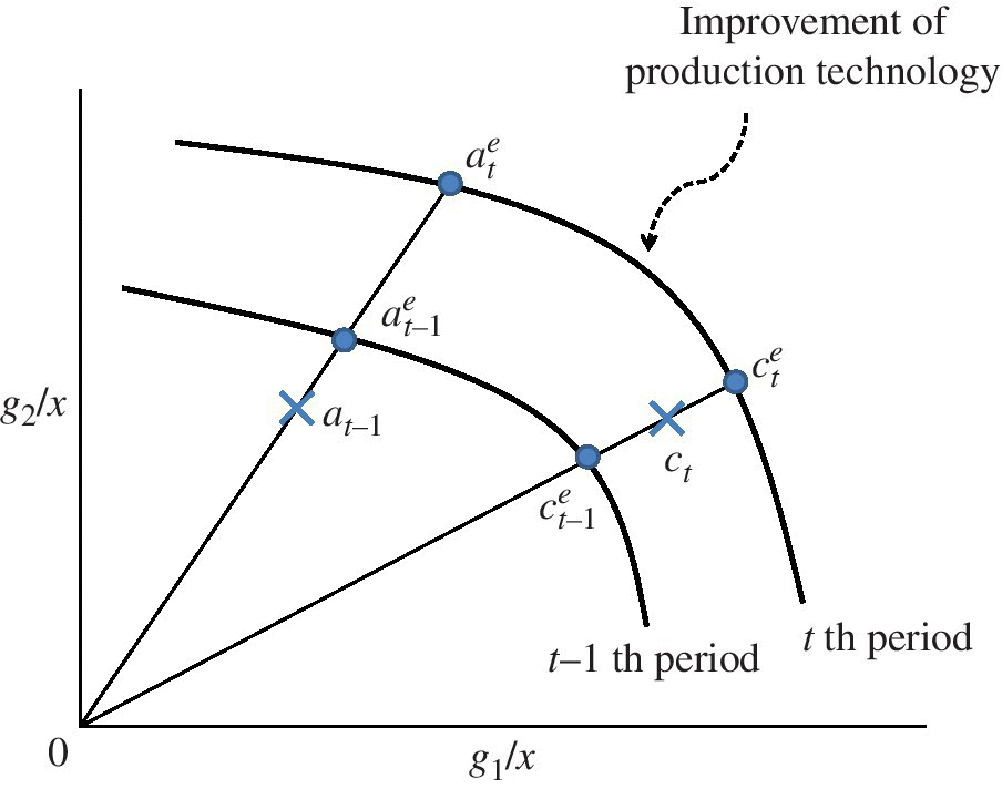
FIGURE 19.1 Frontier shift under natural disposability. (b) The efficiency frontier shifts toward an increase in desirable outputs without any frontier crossover between the two periods. The natural disposability implies that the first priority is operational performance and the second priority is environmental performance. The figure assumes that an undesirable output (b) is same for all DMUs, so reducing the influence on a frontier shift. (c) The figure assumes that DEA does not suffer from an occurrence of multiple projections and multiple reference sets. (d) A unique projection onto the two efficiency frontiers is for our visual convenience. This chapter fully understands that a real projection in DEA is more complicated than the one depicted in the figure. (e) As discussed in Chapter 3, this chapter clearly understands that the projection should be measured by the L1‐metric distance, not the L2‐metric distance, as depicted in the figure. Such a metric change is for our visual convenience.
(a) Source: Sueyoshi and Goto (2013c)
In Figure 19.1, ![]() stands for the observed performance of a DMU at the t–1 th period. Meanwhile, ct indicates the observed performance of the DMU at the t th period for t = 2,…,T. The symbol (0) stands for an origin in the figure. A frontier shift occurs toward the north‐east direction under the assumption that a technology progress on desirable outputs occur between the two periods. A shift toward the north‐east direction is due to performance betterment under natural disposability. Figure 19.1 assumes that the amount of undesirable outputs is the same between the two periods.
stands for the observed performance of a DMU at the t–1 th period. Meanwhile, ct indicates the observed performance of the DMU at the t th period for t = 2,…,T. The symbol (0) stands for an origin in the figure. A frontier shift occurs toward the north‐east direction under the assumption that a technology progress on desirable outputs occur between the two periods. A shift toward the north‐east direction is due to performance betterment under natural disposability. Figure 19.1 assumes that the amount of undesirable outputs is the same between the two periods.
The performance of ![]() is projected to
is projected to ![]() on the efficiency frontier in the t–1 th period and
on the efficiency frontier in the t–1 th period and ![]() on the efficiency frontier in the t th period, respectively, where the superscript e implies an efficiency frontier on which observed performance is projected. In the two cases, this chapter assumes a unique projection and a unique reference set in the two periods, as visually described in Figure 19.1. Under the same assumption, the performance of ct is projected to
on the efficiency frontier in the t th period, respectively, where the superscript e implies an efficiency frontier on which observed performance is projected. In the two cases, this chapter assumes a unique projection and a unique reference set in the two periods, as visually described in Figure 19.1. Under the same assumption, the performance of ct is projected to ![]() on the efficiency frontier for the t–1 th period and
on the efficiency frontier for the t–1 th period and ![]() on the efficiency frontier for the t th period, respectively.
on the efficiency frontier for the t th period, respectively.
A geometric mean, which is widely used to measure the average of the two line segments (![]() and
and ![]() ), indicates the degree of a frontier shift between the t–1 th and t th periods. The geometric mean, indicating a “Malmquist index,” is expressed by the following subcomponents:
), indicates the degree of a frontier shift between the t–1 th and t th periods. The geometric mean, indicating a “Malmquist index,” is expressed by the following subcomponents:
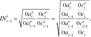
where ![]() stands for the Malmquist index between the t–1 th and t th periods under natural disposability. Equation (19.1) indicates “Malmquist” index, but the above abbreviation does not use M to express
stands for the Malmquist index between the t–1 th and t th periods under natural disposability. Equation (19.1) indicates “Malmquist” index, but the above abbreviation does not use M to express ![]() because this chapter uses M to express managerial disposability.
because this chapter uses M to express managerial disposability.
Shifting our description from natural disposability to managerial disposability, Figure 19.2 depicts a frontier shift from the t–1 th period to the t th period in which each DMU attempts to enhance environmental performance as the first priority and the operational performance as the second priority. For our visual description, Figure 19.2 considers a single input (x) and two undesirable outputs (b1 and b2). It is assumed that all the DMUs have produced a same amount of a desirable output (g), so that it is not depicted in the figure. In Figure 19.2, ![]() stands for the observed performance of a DMU in the t–1 th period. Meanwhile, qt indicates the observed performance of the DMU in the t th period. A frontier shift occurs toward the south‐west direction under the assumption that an eco‐technology progress (e.g. clean coal technology for electricity generation) on undesirable outputs occur between the two periods. A shift toward the south‐west direction is due to managerial disposability.
stands for the observed performance of a DMU in the t–1 th period. Meanwhile, qt indicates the observed performance of the DMU in the t th period. A frontier shift occurs toward the south‐west direction under the assumption that an eco‐technology progress (e.g. clean coal technology for electricity generation) on undesirable outputs occur between the two periods. A shift toward the south‐west direction is due to managerial disposability.
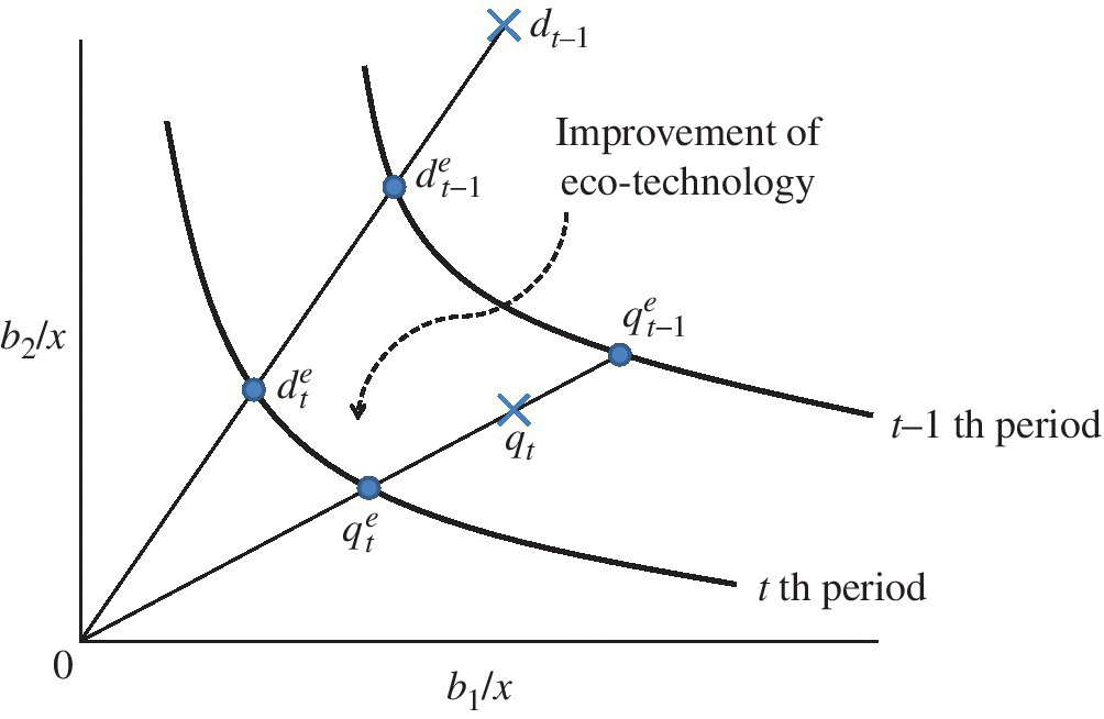
FIGURE 19.2 Frontier shift under managerial disposability. (b) The efficiency frontier shifts toward a decrease in undesirable outputs without any frontier crossover between the two periods. The managerial disposability implies that the first priority is environmental performance and the second priority is operational performance. The figure assumes that desirable outputs are same on all DMUs, so dropping an influence on the frontier shift. (c) See the notes for Figure 19.1.
(a) Source: Sueyoshi and Goto (2013c)
The performance of ![]() can be projected to
can be projected to ![]() on the efficiency frontier for the t–1 th period and
on the efficiency frontier for the t–1 th period and ![]() on the efficiency frontier for the t th period, respectively, in Figure 19.2. Meanwhile, the performance of qt can be projected to
on the efficiency frontier for the t th period, respectively, in Figure 19.2. Meanwhile, the performance of qt can be projected to ![]() on the efficiency frontier of the t–1 th period and
on the efficiency frontier of the t–1 th period and ![]() on the efficiency frontier of the t th period, respectively. The Malmquist index, which measures the geometric mean of the two line segments (
on the efficiency frontier of the t th period, respectively. The Malmquist index, which measures the geometric mean of the two line segments (![]() and
and ![]() ), is expressed by the following subcomponents:
), is expressed by the following subcomponents:
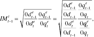
where ![]() stands for the Malmquist index between the t–1 th and t th periods under managerial disposability.
stands for the Malmquist index between the t–1 th and t th periods under managerial disposability.
19.3.2 Occurrence of Frontier Crossover
Figure 19.3, corresponding to Figure 19.1, depicts a possible occurrence of the frontier crossover between the t–1 th and t th periods. The performance of DMUs in Figure 19.3 is measured by natural disposability. In Figure 19.3, an efficiency frontier retreats between the two periods. As a result, it is necessary to combine the two frontiers to shape a new efficiency frontier, or the dotted line in Figure 19.3. To attain the status of efficiency, ![]() and ct need to shift their locations to
and ct need to shift their locations to ![]() and
and ![]() on the newly shaped efficiency frontier.
on the newly shaped efficiency frontier.
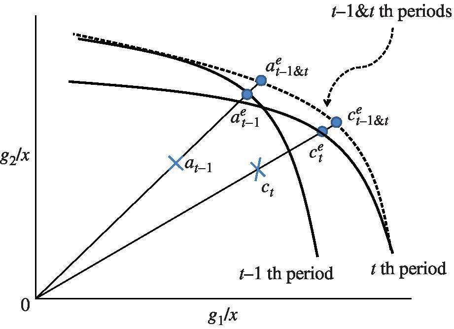
FIGURE 19.3 Frontier crossover between two periods under natural disposability. (b) See the notes for Figure 19.1. (c) The dotted line of the upper curve indicates the frontier for the t–1 th and t th periods.
(a) Source: Sueyoshi and Goto (2013c)
The geometric mean measures the average of the two line segments (![]() and
and ![]() ), indicating the degree of a frontier shift between the t–1 th and t th periods. The geometric mean in this case is expressed by the following notation:
), indicating the degree of a frontier shift between the t–1 th and t th periods. The geometric mean in this case is expressed by the following notation:
where ![]() stands for the Malmquist index between the t–1 th and t th periods under natural disposability, considering a possible occurrence of the frontier crossover (C) between the two periods.
stands for the Malmquist index between the t–1 th and t th periods under natural disposability, considering a possible occurrence of the frontier crossover (C) between the two periods.
In similar manner, Figure 19.4, corresponding to Figure 19.2, visually describes a frontier crossover between the t–1 th and t th periods. In this figure, ![]() and qt need to shift their locations to the projected points,
and qt need to shift their locations to the projected points, ![]() and
and ![]() , on the newly shaped efficiency frontier, or the dotted line for the enhancement of their environmental performance.
, on the newly shaped efficiency frontier, or the dotted line for the enhancement of their environmental performance.
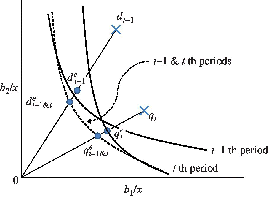
FIGURE 19.4 Frontier crossover between two periods under managerial disposability. (b) See the notes for Figure 19.2. (c) The dotted line of the bottom curve indicates the frontier for the t–1 th and t th periods.
(a) Source: Sueyoshi and Goto (2013c)
The geometric mean in this case measures the average of the two line segments (![]() and
and ![]() ), indicating the degree of a frontier shift between the t–1 th and t th periods. The geometric mean is expressed by the following subcomponents:
), indicating the degree of a frontier shift between the t–1 th and t th periods. The geometric mean is expressed by the following subcomponents:
where ![]() stands for the Malmquist index between the t–1 th and the t th periods under managerial disposability, considering a possible occurrence of the frontier crossover between the two periods.
stands for the Malmquist index between the t–1 th and the t th periods under managerial disposability, considering a possible occurrence of the frontier crossover between the two periods.
It is important to note two concerns. One concern is that the performance of all DMUs at the t th period depends upon only that of the t–1 th and t th periods, not the other periods, as depicted in Figures 19.3 and 19.4. Such a relationship is used for our visual convenience. However, it is not difficult for us to increase the number of periods in the proposed formulations. We can deal with an occurrence of the frontier crossover not only between the adjacent (t–1 th and t th) periods but also among all other period combinations. The other concern is that Equations (19.3) and (19.4) have an analytical benefit, compared with Equations (19.1) and (19.2). That is, we can measure the four components related to a frontier shift by Equations (19.3) and (19.4) even if a frontier crossover occurs between two periods. Meanwhile, Equations (19.1) and (19.2) do not incorporate such an occurrence of the frontier crossover.
19.4 FORMULATIONS FOR NATURAL DISPOSABILITY
The six components to measure ![]() and
and ![]() include
include
 (unified efficiency in the t–1 th period),
 (unified efficiency in the t th period),
 (inter‐temporal unified index from the t–1 th to the t th period),
 (inter‐temporal unified index from the t th period to the t–1 th period),
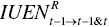 (inter‐temporal unified efficiency from the t–1 th to the t–1 th & t th periods) and
 (inter‐temporal unified efficiency from the t th period to the t–1 th & t th periods.
All efficiency and index measures are determined by radial (R) measurement under natural (N) disposability and constant RTS.
19.4.1 No Occurrence of Frontier Crossover
To measure the Malmquist index under natural disposability in a time horizon (t = 2,…,T), this chapter considers n DMUs ( j = 1,…,n) whose operational and environmental achievements are relatively compared with others in their performance assessment. The performance comparison among multiple periods needs to add subscripts (t) to J so that Jt stands for all DMUs in the t th period.
Returning to Figure 19.1, which depicts a frontier shift with a technology progress, the Malmquist index between the two periods can be restructured as follows:
where ![]() and
and ![]() are two efficiency measures that belong to a range between zero (full inefficiency) and one (full efficiency). Meanwhile,
are two efficiency measures that belong to a range between zero (full inefficiency) and one (full efficiency). Meanwhile, ![]() and
and ![]() may become larger or smaller than unity, depending upon an occurrence of a frontier crossover between the two periods.
may become larger or smaller than unity, depending upon an occurrence of a frontier crossover between the two periods.
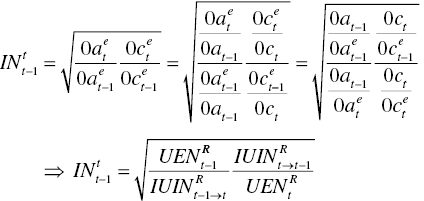
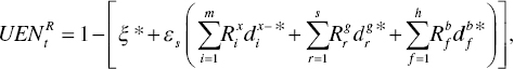
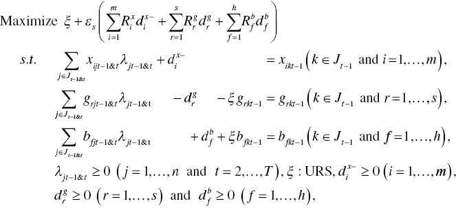
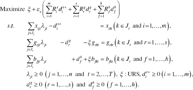
These measures can be formulated by the four DEA models, each of which is specified as follows: First, the degree of ![]() on the k‐th DMU in the t th period (t = 2,…, T) is measured by the following model under natural disposability and constant RTS and DTS:
on the k‐th DMU in the t th period (t = 2,…, T) is measured by the following model under natural disposability and constant RTS and DTS:
where ![]() (i = 1,…,m),
(i = 1,…,m), ![]() (r = 1,…,s) and
(r = 1,…,s) and ![]() (f = 1,…,h) are all slack variables related to inputs, desirable outputs and undesirable outputs, respectively.
(f = 1,…,h) are all slack variables related to inputs, desirable outputs and undesirable outputs, respectively. ![]() is a column vector of unknown variables, often referred to as “structural” or “intensity” variables, that are used for connecting production factors. An unknown scalar value (ξ), which is unrestricted (URS), stands for an inefficiency measure. The inefficiency measure corresponds to a distance between an efficiency frontier and an observed vector of desirable and undesirable outputs, as depicted in Figures 19.1 and 19.2. A scalar value (εs) is also incorporated into Model (19.6) and it stands for a very small number to indicate the relative importance between the inefficiency score and the total amount of slacks. This chapter sets εs = 0.0001 for our computation. The selection is subjective. It is possible for us to set εs = 0. In the case, it is necessary to depend upon a method for multiplier restriction (e.g., cone ratio) or the incorporation of strong complementary slackness conditions (SCSCs) because dual variables may become zero in these magnitudes. That is problematic in DEA because corresponding production factors are not fully utilized in the efficiency assessment. See Chapter 7 for a description on how to handle the difficulty by SCSCs.
is a column vector of unknown variables, often referred to as “structural” or “intensity” variables, that are used for connecting production factors. An unknown scalar value (ξ), which is unrestricted (URS), stands for an inefficiency measure. The inefficiency measure corresponds to a distance between an efficiency frontier and an observed vector of desirable and undesirable outputs, as depicted in Figures 19.1 and 19.2. A scalar value (εs) is also incorporated into Model (19.6) and it stands for a very small number to indicate the relative importance between the inefficiency score and the total amount of slacks. This chapter sets εs = 0.0001 for our computation. The selection is subjective. It is possible for us to set εs = 0. In the case, it is necessary to depend upon a method for multiplier restriction (e.g., cone ratio) or the incorporation of strong complementary slackness conditions (SCSCs) because dual variables may become zero in these magnitudes. That is problematic in DEA because corresponding production factors are not fully utilized in the efficiency assessment. See Chapter 7 for a description on how to handle the difficulty by SCSCs.
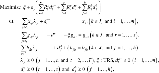
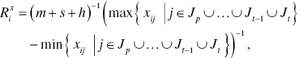
The data range adjustments in Model (19.6) are determined by the upper and lower bounds of production factors. These upper and lower bounds are specified by
Here, ![]() stands for a union set. Thus,
stands for a union set. Thus, ![]() stands for all DMUs in the t–1 th and t th periods.
stands for all DMUs in the t–1 th and t th periods.
The degree of ![]() of the k‐th DMU in the t th period is determined by
of the k‐th DMU in the t th period is determined by
where the inefficiency score and all slack variables are determined on the optimality of Model (19.6). The equation within the parenthesis, obtained from the optimality of Model (19.6), indicates the level of unified inefficiency under natural disposability. The unified efficiency is obtained by subtracting the level of unified inefficiency from unity. The degree of ![]() on the k‐th DMU is always less than unity, indicating an existence of some level of inefficiency, or equal unity for the status of full efficiency.
on the k‐th DMU is always less than unity, indicating an existence of some level of inefficiency, or equal unity for the status of full efficiency.
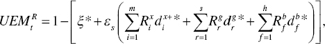
Second, the degree of ![]() regarding the k‐th DMU in the t–1 th period is measured by replacing t by t–1 in Model (19.6). Then, the degree is measured by Equation (19.7) as follows:
regarding the k‐th DMU in the t–1 th period is measured by replacing t by t–1 in Model (19.6). Then, the degree is measured by Equation (19.7) as follows:
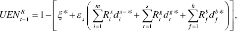
where the inefficient score and slacks on optimality are measured by Model (19.6) after replacing t by t–1 in the formulation.
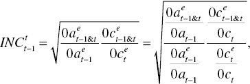
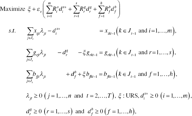
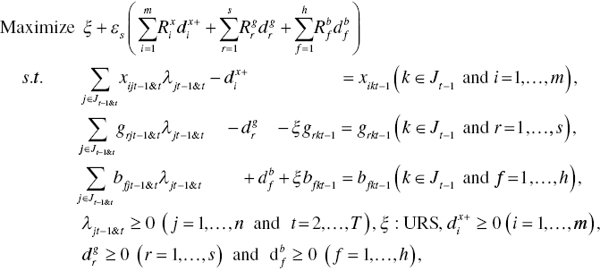
Third, the degree of ![]() regarding the k‐th DMU from the t–1 th period to the t th period is determined by the following model:
regarding the k‐th DMU from the t–1 th period to the t th period is determined by the following model:
where an efficiency frontier consists of DMUs in the t th period and a DMU to be examined is selected from a group of DUMs in the t–1 th period. The degree of the index is measured by Equation (19.7) where the inefficiency measure and all slack variables are determined on optimality of Model (19.8).
The degree of ![]() regarding the k‐th DMU that shifts from the t th period to the t–1 th period is determined by the following model:
regarding the k‐th DMU that shifts from the t th period to the t–1 th period is determined by the following model:
where an efficiency frontier consists of DMUs in the t–1 th period and a DMU to be examined is selected from a group of DUMs in the t th period. The degree of the index is measured by Equation (19.7) where the inefficiency measure and all slack variables are determined on optimality of Model (19.9).
19.4.2 Occurrence of Frontier Crossover
Returning to Figure 19.3, the conceptual framework for Equation (19.3) under natural disposability is expressed by the following measures in the case of a frontier crossover:
where ![]() is separated into four subcomponents, all of which are used to measure a frontier shift between the two periods (i.e.,
is separated into four subcomponents, all of which are used to measure a frontier shift between the two periods (i.e., ![]() ,
, ![]() ,
, ![]() and
and ![]() ). Among the four subcomponents, this chapter has already discussed the measurement of
). Among the four subcomponents, this chapter has already discussed the measurement of ![]() and
and ![]() , so focusing upon the remaining measurement of
, so focusing upon the remaining measurement of ![]() and
and ![]() , hereafter.
, hereafter.
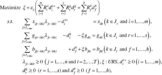
The degree of ![]() regarding the k‐th DMU between the two periods is determined by the following model:
regarding the k‐th DMU between the two periods is determined by the following model:
where an efficiency frontier consists of DMUs in the t–1 th and t th periods and a DMU to be examined by Model (19.11) is selected from a group of DUMs in the t–1 th period. The degree of ![]() on the k‐th DMU is determined by Equation (19.7) where the inefficiency measure and all slack variables are determined on the optimality of Model (19.11).
on the k‐th DMU is determined by Equation (19.7) where the inefficiency measure and all slack variables are determined on the optimality of Model (19.11).
The degree of ![]() on the k‐th DMU between the two periods is determined by the following model:
on the k‐th DMU between the two periods is determined by the following model:
where an efficiency frontier consists of DMUs in the t–1 th and t th periods and a DMU to be examined is selected from DUMs in the t th period. The degree of ![]() regarding the k‐th DMU in the t th period is determined by Equation (19.7) where the inefficiency measure and all slack variables are determined on the optimality of Model (19.12).
regarding the k‐th DMU in the t th period is determined by Equation (19.7) where the inefficiency measure and all slack variables are determined on the optimality of Model (19.12).
At the end of this section, it is necessary to describe two differences between index and efficiency measures. One of the two differences is that as a result of incorporating a frontier crossover in Models (19.11) and (19.12), the two models always produce efficiency scores, not indexes, which belong to a range between 0 (full inefficiency) and 1 (full efficiency). Such a feature cannot be found in Models (19.8) and (19.9). The other difference is that ![]() may be more than, equal to or less than unity, but
may be more than, equal to or less than unity, but ![]() is more than or equal to unity and it cannot be less than unity. If a DMU exhibits unity in
is more than or equal to unity and it cannot be less than unity. If a DMU exhibits unity in ![]() , then it indicates that there is a frontier crossover between the t–1 th and t th periods and the achievement of the DMU locates on the three efficiency frontiers for the t–1 th, t th and the combined t–1 th and t th periods. In other words, there is no technological progress between the two periods. In contrast, if a DMU exhibits more than unity in
, then it indicates that there is a frontier crossover between the t–1 th and t th periods and the achievement of the DMU locates on the three efficiency frontiers for the t–1 th, t th and the combined t–1 th and t th periods. In other words, there is no technological progress between the two periods. In contrast, if a DMU exhibits more than unity in ![]() , then it indicates that the efficiency frontier of the t th period locates differently from that of the t–1 th period, as depicted in Figure 19.3. Thus, it is possible for us to identify whether the DMU has an operational improvement (e,g., due to technological progress) or an operational retreat (e.g,, due to poor business condition) between the two periods by examining
, then it indicates that the efficiency frontier of the t th period locates differently from that of the t–1 th period, as depicted in Figure 19.3. Thus, it is possible for us to identify whether the DMU has an operational improvement (e,g., due to technological progress) or an operational retreat (e.g,, due to poor business condition) between the two periods by examining ![]() . Finally, it is important to note that our description here is based upon the assumption that a data set to be examined does not contain an outlier because it drastically changes the location of an efficiency frontier. See Chapter 2 on a description on an outlier.
. Finally, it is important to note that our description here is based upon the assumption that a data set to be examined does not contain an outlier because it drastically changes the location of an efficiency frontier. See Chapter 2 on a description on an outlier.
19.5 FORMULATIONS UNDER MANAGERIAL DISPOSABILITY
To describe the six components regarding ![]() and
and ![]() , this chapter specifies their subcomponents as follows:
, this chapter specifies their subcomponents as follows:
 (unified efficiency in the t–1 th period),
 (unified efficiency in the t th period),
 (inter‐temporal unified index from the t–1 th to the t th period),
 (inter‐temporal unified index from the t th to the t–1 th period),
 (inter‐temporal unified efficiency from the t–1 th to the t–1 th & t th periods), and
 (inter‐temporal unified efficiency from the t th to the t–1 th & t th periods).
All efficiency and index measures are determined by radial measurement under managerial (M) disposability and constant DTS.
19.5.1 No Occurrence of Frontier Crossover
The conceptual framework in Equation (19.2), or ![]() under managerial disposability, is expressed by the following subcomponents as depicted in Figure 19.2:
under managerial disposability, is expressed by the following subcomponents as depicted in Figure 19.2:
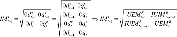
As formulated in Equation (19.13), ![]() is separated into four subcomponents, all of which are measured under constant DTS.
is separated into four subcomponents, all of which are measured under constant DTS.
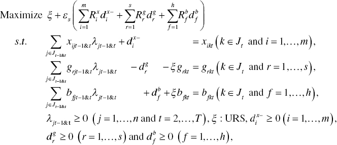
First, the degree of ![]() of the k‐th DMU in the t th period is measured by the following model:
of the k‐th DMU in the t th period is measured by the following model:
The degree of ![]() regarding the k‐th DMU in the t th period is determined by
regarding the k‐th DMU in the t th period is determined by
where the inefficiency score and all slack variables are determined on the optimality of Model (19.14). The equation within the parenthesis, obtained from the optimality of Model (19.14), indicates the level of unified inefficiency under managerial disposability. The unified efficiency is obtained by subtracting the level of inefficiency from unity. Thus, the unified efficiency always belongs to the range between 0 (full inefficiency) and 1 (full efficiency).
Second, the degree of ![]() regarding the k‐th DMU at the t–1 th period is measured by replacing t by t–1 in Model (19.14). Equation (19.15) is used to measure the degree of
regarding the k‐th DMU at the t–1 th period is measured by replacing t by t–1 in Model (19.14). Equation (19.15) is used to measure the degree of ![]() after replacing t by t–1 in Model (19.14).
after replacing t by t–1 in Model (19.14).
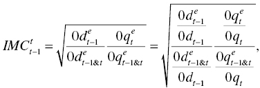
Third, the degree of ![]() of the k‐th DMU from the t–1 th period to the t th period is determined by the following model:
of the k‐th DMU from the t–1 th period to the t th period is determined by the following model:
where an efficiency frontier consists of DMUs in the t th periods and a DMU to be examined is selected from DUMs in the t–1 th period. The degree of ![]() of the k‐th DMU is measured by Equation (19.15) where the inefficiency measure and all slack variables are determined on the optimality of Model (19.16).
of the k‐th DMU is measured by Equation (19.15) where the inefficiency measure and all slack variables are determined on the optimality of Model (19.16).
The degree of ![]() of the k‐th DMU from the t th to the t–1 th period is determined by the following model:
of the k‐th DMU from the t th to the t–1 th period is determined by the following model:
where an efficiency frontier consists of DMUs in the t–1 th period and a DMU to be examined is selected from a group of DUMs in the t th period. The degree of ![]() on the k‐th DMU between the two periods is measured by Equation (19.15) where the inefficiency measure and all slack variables are determined on optimality of Model (19.17).
on the k‐th DMU between the two periods is measured by Equation (19.15) where the inefficiency measure and all slack variables are determined on optimality of Model (19.17).
19.5.2 Occurrence of Frontier Crossover
By shifting our description to the case of a frontier crossover, the conceptual framework on Equation (19.4), or ![]() , under managerial disposability, is expressed by the following unified measures as depicted in Figure 19.4:
, under managerial disposability, is expressed by the following unified measures as depicted in Figure 19.4:
The degree of ![]() and that of
and that of ![]() are measured by Model (19.14). The first measurement needs to replace the t th by the t–1 th period in the model.
are measured by Model (19.14). The first measurement needs to replace the t th by the t–1 th period in the model.
The degree of ![]() of the k‐th DMU in the t–1 th period is determined by the following model:
of the k‐th DMU in the t–1 th period is determined by the following model:
where an efficiency frontier consists of DMUs in the t–1 th and t th periods and a DMU to be examined is selected from DUMs in the t–1 th period. The degree of ![]() of the k‐th DMU is measured by Equation (19.15) where the inefficiency score and all slack variables are determined on the optimality of Model (19.19).
of the k‐th DMU is measured by Equation (19.15) where the inefficiency score and all slack variables are determined on the optimality of Model (19.19).
The degree of ![]() of the k‐th DMU in the t th period is determined by the following model:
of the k‐th DMU in the t th period is determined by the following model:
where an efficiency frontier consists of DMUs in the t–1 th and t th periods and a DMU to be examined is selected from a group of DUMs in the t th period. The degree of ![]() is measured by Equation (19.15) where the inefficiency score and all slack variables are determined on the optimality of the model in Equation (19.20). As a result of incorporating an occurrence of a frontier shift in Models (19.19) and (19.20), the two models can always produce an efficiency score on a range between 0 (full inefficiency) and 1 (full efficiency). Such a feature cannot be found in Models (19.16) and (19.17).
is measured by Equation (19.15) where the inefficiency score and all slack variables are determined on the optimality of the model in Equation (19.20). As a result of incorporating an occurrence of a frontier shift in Models (19.19) and (19.20), the two models can always produce an efficiency score on a range between 0 (full inefficiency) and 1 (full efficiency). Such a feature cannot be found in Models (19.16) and (19.17).
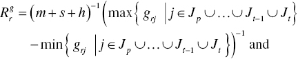
The proposed Malmquist index measurement under natural or managerial disposability has the four important features discussed here. First, all the models are formulated under constant RTS and DTS. It is impossible to measure the indexes under variable RTS and DTS because we must face an infeasible solution. See Chapter 6 for the mathematical property. Second, this chapter assumes that all DEA models in Sections 19.3 and 19.4 can uniquely produce a DEA solution. However, the assumption is not always true because they may suffer from an occurrence of multiple solutions (e.g., multiple projections and reference sets). If such a problem occurs, it is necessary to incorporate SCSCs to the proposed DEA models for a time horizon. Third, this chapter considers only two periods (t–1 and t) in discussing the occurrence of a frontier crossover between the two periods. It is possible for us to extend the number of periods to more than three periods (![]() ), where the subscript (p) indicates a starting period of the window. See Sueyoshi and Goto (2015). In the case of multiple (more than two) periods, the data ranges (R) are determined by the upper and lower bounds of production factors as follows:
), where the subscript (p) indicates a starting period of the window. See Sueyoshi and Goto (2015). In the case of multiple (more than two) periods, the data ranges (R) are determined by the upper and lower bounds of production factors as follows:
Finally, many production economists (e.g., Zhou et al. 2012a) used a directional distance function to express the analytical structure for inefficiency measurement. This chapter does not follow such a conventional way of measurement because of a difficulty in mathematically describing a frontier crossover between different periods and different technology developments. Further, the use of conventional distance functions has implicitly assumed a unique solution on DEA. In contrast, this chapter formulates DEA models as linear programming, so that they may suffer from an occurrence of multiple solutions in their primal and dual models.
19.6 ENERGY MIX OF INDUSTRIAL NATIONS
This chapter sampled ten industrial nations from the OECD countries whose energy structures are characterized by three inputs (i.e., the net electrical capacity of main producer plants with respect to combustible, nuclear, hydro and renewable energies), a single desirable output (i.e, the total net production of electricity) and a single undesirable output (i.e., the amount of CO2 emissions from fuel combustion of main electric power plants). The two units MWe and GWh stand for Megawatt electric and Gigawatt hour, respectively.
Data Accessibility:
The data sources used in this chapter are OECD statistics such as (a) IEA electricity information statistics, OECD net electrical capacity, total main activity producer plants (containing inputs), (b) IEA electricity information statistics, OECD electricity/heat supply and consumption, electricity, total net production (containing a desirable output), and (c) IEA CO2 emissions from fuel combustion statistics, detailed CO2 estimates, main activity electricity plants, total (containing an undesirable output; CO2 emission). Here, IEA stands for International Energy Agency.
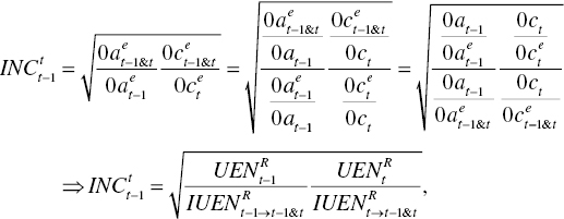
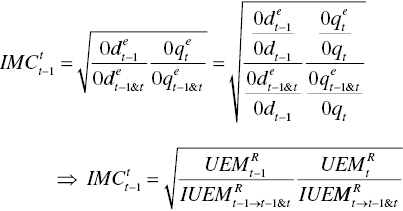
Table 19.1 summarizes the Malmquist indexes (![]() ) of the ten nations which are measured under natural disposability under the assumption that a frontier crossover has not occurred in the observed period (2000–2009). In a similar manner, Table 19.2 summarizes the indexes (
) of the ten nations which are measured under natural disposability under the assumption that a frontier crossover has not occurred in the observed period (2000–2009). In a similar manner, Table 19.2 summarizes the indexes (![]() ) under the assumption that a frontier crossover has occurred between the adjacent annual periods. Note that unified efficiency measures (
) under the assumption that a frontier crossover has occurred between the adjacent annual periods. Note that unified efficiency measures (![]() ) under natural disposability are summarized in Sueyoshi and Goto (2013c).
) under natural disposability are summarized in Sueyoshi and Goto (2013c).
TABLE 19.1 Malmquist index under natural disposability: no frontier crossover
(a) Source: Sueyoshi and Goto (2013c).
| Canada | France | Germany | Japan | Korea | Mexico | Netherlands | Spain | United Kingdom | United States | |
| 2000 | 1.0183 | 1.0191 | 1.0706 | 1.0374 | 1.1030 | 1.0403 | 0.9915 | 1.0544 | 1.0706 | 1.0587 |
| 2001 | 0.9708 | 1.0576 | 1.0109 | 1.0198 | 0.9764 | 0.9986 | 1.0109 | 0.9881 | 1.0256 | 0.9479 |
| 2002 | 1.0191 | 0.9801 | 1.0037 | 1.0109 | 1.0244 | 0.9665 | 0.9221 | 1.0150 | 0.9992 | 0.9968 |
| 2003 | 0.9563 | 0.9922 | 1.0074 | 0.9952 | 1.0161 | 0.9356 | 0.9115 | 0.9648 | 1.0213 | 1.0175 |
| 2004 | 0.9585 | 1.0144 | 0.9954 | 1.0169 | 1.0108 | 1.0536 | 0.9812 | 1.0301 | 1.0015 | 1.0277 |
| 2005 | 1.0159 | 1.0193 | 1.0150 | 1.0061 | 1.0234 | 1.0378 | 0.9433 | 1.0416 | 0.9388 | 0.9828 |
| 2006 | 0.9826 | 1.0495 | 0.9715 | 0.9789 | 0.9164 | 0.9851 | 0.9320 | 1.0127 | 0.9947 | 0.9529 |
| 2007 | 1.0154 | 0.9808 | 1.0374 | 1.0306 | 1.0093 | 1.0111 | 1.0285 | 1.0111 | 0.9096 | 1.0822 |
| 2008 | 1.0114 | 0.9804 | 0.9774 | 0.9795 | 0.9658 | 1.0261 | 0.9451 | 1.0341 | 0.9376 | 0.9717 |
| 2009 | 0.9378 | 0.9018 | 0.9369 | 0.9558 | 0.9844 | 0.9835 | 1.0122 | 1.0445 | 0.9788 | 0.9872 |
TABLE 19.2 Malmquist index under natural disposability: frontier crossover
(a) Source: Sueyoshi and Goto (2013c).
| Canada | France | Germany | Japan | Korea | Mexico | Netherlands | Spain | United Kingdom | United States | |
| 2000 | 1.0000 | 1.0000 | 1.0398 | 1.0184 | 1.0242 | 1.0113 | 1.0000 | 1.0263 | 1.0321 | 1.0203 |
| 2001 | 1.0095 | 1.0000 | 1.0163 | 1.0171 | 1.0000 | 1.0000 | 1.0000 | 1.0191 | 1.0121 | 1.0208 |
| 2002 | 1.0022 | 1.0000 | 1.0014 | 1.0052 | 1.0000 | 1.0112 | 1.0000 | 1.0071 | 1.0025 | 1.0029 |
| 2003 | 1.0143 | 1.0000 | 1.0162 | 1.0090 | 1.0025 | 1.0309 | 1.0000 | 1.0193 | 1.0133 | 1.0169 |
| 2004 | 1.0000 | 1.0000 | 1.0110 | 1.0153 | 1.0000 | 1.0265 | 1.0000 | 1.0150 | 1.0160 | 1.0220 |
| 2005 | 1.0012 | 1.0000 | 1.0149 | 1.0116 | 1.0069 | 1.0149 | 1.0000 | 1.0214 | 1.0528 | 1.0257 |
| 2006 | 1.0030 | 1.0000 | 1.0154 | 1.0116 | 1.0066 | 1.0020 | 1.0000 | 1.0111 | 1.0021 | 1.0246 |
| 2007 | 1.0016 | 1.0038 | 1.0183 | 1.0191 | 1.0000 | 1.0000 | 1.0000 | 1.0068 | 1.0133 | 1.0410 |
| 2008 | 1.0000 | 1.0000 | 1.0106 | 1.0100 | 1.0025 | 1.0110 | 1.0000 | 1.0180 | 1.0228 | 1.0148 |
| 2009 | 1.0000 | 1.0444 | 1.0402 | 1.0250 | 1.0000 | 1.0070 | 1.0000 | 1.0229 | 1.0170 | 1.0177 |
The index measures provide two interesting findings. One of the two findings is that the electric power industry is a huge process industry whose investment in new technology requires a large amount of capital. The speed of technology innovation on generation (as a desirable output) is relatively slow so that the Malmquist index measures fluctuate around unity until a generation system can completely utilize the new technology. Consequently, Table 19.1 (under the assumption of no frontier crossover) cannot catch the influence of technology innovation. Meanwhile, Table 19.2 (under an occurrence of the crossover between two adjacent periods) can identify such a frontier shift with the indexes more than or equal to unity although the speed and degree of technology innovation are still very modest.
According to the research of Sueyoshi and Goto (2013c), France has been utilizing nuclear energy to generate electricity and to reduce the amount of CO2 emission. The Netherlands uses hydro and renewable generations. The performance of France indicates that the nuclear power generation may be important in developing a sustainable society with low CO2 emission. It is indeed true that we need to pay attention to renewable energy sources, as well. However, their generation outputs are significantly small, compared with that of nuclear generation. A shortcut to establishing a sustainable society may depend upon the use of nuclear power generation until we can access advanced technology on renewable generation with reasonable costs. This concern on electricity generation does not imply that this chapter denies the importance of renewable energy sources. As found in the Netherlands, it is possible for us to fully utilize a combination between hydro‐generation and renewable energy (e.g., solar and wind) for electricity generation and reduction of CO2 emissions. It is easily envisioned that the use of hydro and renewable energy will be able to contribute to the development of a sustainable society. However, it is important for us to consider each nation’s geographic features and historical development of generation capacities for optimal fuel mix strategy.
Table 19.3 summarizes the Malmquist indexes (![]() ) of the ten nations which are measured under managerial disposability under the assumption that a crossover of efficiency frontiers has not occurred in the observed periods (2000‐2009). In a similar manner, Table 19.4 summarizes the indexes (
) of the ten nations which are measured under managerial disposability under the assumption that a crossover of efficiency frontiers has not occurred in the observed periods (2000‐2009). In a similar manner, Table 19.4 summarizes the indexes (![]() ) under the assumption that a frontier crossover has occurred between two adjacent (t–1 th and t th) periods. Note that unified efficiency measures (
) under the assumption that a frontier crossover has occurred between two adjacent (t–1 th and t th) periods. Note that unified efficiency measures (![]() ) under managerial disposability are summarized in Sueyoshi and Goto (2013c).
) under managerial disposability are summarized in Sueyoshi and Goto (2013c).
TABLE 19.3 Malmquist index under managerial disposability: no frontier crossover
(a) Source: Sueyoshi and Goto (2013c).
| Canada | France | Germany | Japan | Korea | Mexico | Netherlands | Spain | United Kingdom | United States | |
| 2000 | 1.2223 | 1.1516 | 1.0881 | 1.0736 | 1.0924 | 1.0927 | 1.0203 | 1.1655 | 1.0667 | 1.1079 |
| 2001 | 1.3170 | 1.2622 | 1.2583 | 1.2377 | 1.2746 | 1.2589 | 1.1874 | 1.3317 | 1.2311 | 1.2565 |
| 2002 | 0.8953 | 0.9208 | 0.9101 | 0.9101 | 0.9101 | 0.9101 | 0.9101 | 0.9101 | 0.9101 | 0.9101 |
| 2003 | 0.9169 | 0.9363 | 0.9100 | 0.9100 | 0.9100 | 0.9100 | 0.9100 | 0.9100 | 0.9100 | 0.9100 |
| 2004 | 1.0588 | 1.0565 | 1.0776 | 1.0776 | 1.0776 | 1.0776 | 1.0776 | 1.0776 | 1.0776 | 1.0776 |
| 2005 | 0.8773 | 0.8509 | 0.8390 | 0.8557 | 0.8316 | 0.8584 | 0.8884 | 0.8203 | 0.8624 | 0.8715 |
| 2006 | 1.2951 | 1.2093 | 1.1493 | 1.1350 | 1.1564 | 1.1309 | 1.1052 | 1.1655 | 1.1271 | 1.1203 |
| 2007 | 0.9979 | 0.9834 | 0.9391 | 0.9342 | 0.9417 | 0.9304 | 0.9203 | 0.9435 | 0.9292 | 0.9268 |
| 2008 | 0.9372 | 0.9251 | 0.9964 | 1.0141 | 0.9940 | 1.0274 | 1.0632 | 0.9783 | 1.0328 | 1.0400 |
| 2009 | 0.9059 | 0.9054 | 0.9354 | 0.9366 | 0.9319 | 0.9375 | 0.9435 | 0.9376 | 0.9392 | 0.9400 |
TABLE 19.4 Malmquist index under managerial disposability: frontier crossover
(a) Source: Sueyoshi and Goto (2013c).
| Canada | France | Germany | Japan | Korea | Mexico | Netherlands | Spain | United Kingdom | United States | |
| 2000 | 1.1056 | 1.0416 | 1.0429 | 1.0363 | 1.0395 | 1.0442 | 1.0099 | 1.0769 | 1.0329 | 1.0494 |
| 2001 | 1.1476 | 1.0812 | 1.1201 | 1.1133 | 1.1283 | 1.1231 | 1.0878 | 1.1524 | 1.1094 | 1.1329 |
| 2002 | 1.0568 | 1.0258 | 1.0482 | 1.0482 | 1.0482 | 1.0482 | 1.0482 | 1.0482 | 1.0482 | 1.0482 |
| 2003 | 1.0443 | 1.0189 | 1.0483 | 1.0483 | 1.0483 | 1.0483 | 1.0483 | 1.0483 | 1.0483 | 1.0483 |
| 2004 | 1.0290 | 1.0178 | 1.0381 | 1.0381 | 1.0381 | 1.0381 | 1.0381 | 1.0381 | 1.0381 | 1.0381 |
| 2005 | 1.0676 | 1.0379 | 1.0930 | 1.0820 | 1.0973 | 1.0801 | 1.0596 | 1.1022 | 1.0768 | 1.0713 |
| 2006 | 1.1380 | 1.0627 | 1.0725 | 1.0653 | 1.0753 | 1.0642 | 1.0504 | 1.0796 | 1.0620 | 1.0586 |
| 2007 | 1.0010 | 1.0010 | 1.0316 | 1.0341 | 1.0307 | 1.0368 | 1.0418 | 1.0293 | 1.0374 | 1.0386 |
| 2008 | 1.0330 | 1.0253 | 1.0397 | 1.0364 | 1.0383 | 1.0366 | 1.0313 | 1.0453 | 1.0353 | 1.0346 |
| 2009 | 1.0506 | 1.0344 | 1.0322 | 1.0329 | 1.0361 | 1.0328 | 1.0287 | 1.0328 | 1.0315 | 1.0312 |
The index measures in Tables 19.3 and 19.4 provide two interesting findings. One of the two findings is that the electric power industry has a time lag to establish eco‐technology innovation on CO2 reduction because the electricity generation belongs to a capital‐intensive industry so that the technology innovation needs a large amount of capital investment to reduce the amount of CO2 emission which is required by the government of each nation. Such a unique feature influences the index measures in such a manner that they fluctuate around unity, as in Table 19.3, and the technology innovation, or a frontier shift, becomes very modest, as found in Table 19.4.
19.7 SUMMARY
This chapter discussed a use of the Malmquist index to measure a frontier shift among different periods. A contribution of this chapter was that it made an analytical linkage between the index measurement and the concept of natural or managerial disposability. The Malmquist index measure, discussed in this chapter, was separated into twelve different subcomponents (6 subcomponents x 2 disposability concepts). All subcomponents provided us with information on how much the frontier shift occurred among different periods.
Contributions of the proposed Malmquist index are summarized as follows: The proposed approach incorporates both desirable and undesirable outputs in DEA formulations under natural or managerial disposability. A frontier shift is measurable under the two different disposability concepts within the conceptual framework of Stage I (A) and (B) of Figure 15‐6. This type of unique feature cannot be found in the other indexes.
The frontier shift measurement has three drawbacks. First, the proposed approach belongs to only Stage I, not attaining Stages II and III, of Figure 15‐6 in which disposability concepts are unified under the assumption that undesirable outputs are by‐products of desirable outputs. Moreover, an occurrence of congestion under natural or managerial disposability is the most important concept in DEA environmental assessment. See Chapters 15 and 21. This chapter does not incorporate the occurrence in a time horizon. Second, the proposed approach must assume constant RTS and DTS in the formulations. If the assumption is dropped, then the approach must face an infeasible solution. See Chapter 20. Finally, the proposed approach assumes that all production factors are strictly positive, so that it cannot directly handle an occurrence of zero and/or negative values in a data set. See Chapters 26 and 27 for a description on how to deal with such a data set with zero and/or negative values. No study has been done on such a data set in a time horizon.
The proposed DEA approach identified the three empirical findings on energy, all of which were useful in the green growth development of economy to establish a sustainable society. First, the electric power industry had a time lag until eco‐technology innovation really influenced the amount of generation and the reduction of CO2 emission. That was because the industry needed a large capital investment to introduce new technology for generation and environmental protection. Therefore, it was necessary to consider the existence of a frontier crossover under the assumption that the frontier was formulated by a wider range of combinations of advanced generation technology in a time horizon. Second, nuclear generation as found in France and hydro and renewable energy as found in the Netherlands were important for the development of a sustainable society although the former was associated with a very high level of risk and the latter had a limited generation capability. Finally, the industry had been making a corporate effort to reduce the amount of CO2 emission by utilizing nuclear power and renewable energy although the degree and speed of technology innovation was relatively modest.
Here, it is important to note that nuclear power generation is always associated with very high risk, as found in the disaster at Fukushima Daiichi in March, 2011. See Chapter 26 that discusses the fuel mix strategy of 33 OECD nations after the disaster at the Fukushima Daiichi nuclear power plant. It is a major policy issue for all nations to pay serious attention to various types of security issues in the operation of nuclear power plants. Meanwhile, the utilization of hydro power is limited in its growth because many industrial nations have already developed dams which can generate a large amount of electricity. The development opportunity for large hydro power plants is now limited in many industrial nations. As a result, many nations recently pay attention to renewable energy sources11.
Finally, it is necessary to discuss the importance of balancing between economic prosperity and environmental protection in order to direct each nation toward a sustainable society which can attain a green growth by paying serious attention to environmental protection. To attain a sustainable society, we look forward to seeing future technology development on renewable energy. It is also expected that technology development produces an economic benefit for renewable energy in such a manner that it can compete with the other conventional generation technologies without relying on any financial support scheme such as FIT. Until the development of such a sustainable society, it may be necessary for us to utilize the nuclear power generation as an important component of a fuel mix under a rigorous safety standard in a short time horizon, not a long‐term horizon, where it is hoped that renewable power generation will be more efficient than nuclear power generation.
APPENDIX
There are various types of total factor productivity (TFP) measures. They include all products and services produced and account for all of the resources used to produce these goods and services. The TFP is thus formulated by the ratio of all of desirable outputs produced over all of the inputs employed to produce them. The traditional productivity indexes, such as Laspeyres, Paasche, Fisher and Törnqvist, use price information to allow us to add up the products (desirable outputs) and resources (inputs).
Table 19.A1 briefly summarizes previous indexes. It is clearly understood that each index has strengths and drawbacks. This chapter does not provide a conventional description on them. Rather, this chapter describes two concerns on them from the perspective of implementing the proposed DEA environmental assessment. One concern is that desirable and undesirable outputs should be incorporated in the computational framework. Then, it is necessary for us to discuss how to unify them in measuring indexes. The other concern is that the proposed formulations for the assessment need to incorporate a possible occurrence of undesirable or desirable congestion. The desirable congestion is important in measuring eco‐technology development in a time horizon. The previous index theory did not incorporate such two important concerns. Thus, they are very limited in their applicability when discussing the issue of sustainability.
TABLE 19.A1 Popular indexes for productivity measurement
(a) Outputs in the table imply desirable outputs. No previous article has separated outputs into desirable and undesirable categories. (b) This chapter does not use the econometric distance function for measuring Malmquist index. The separation between desirable and undesirable outputs is incorporated into the proposed DEA approach in a time horizon. Thus, the proposed approach follows the conceptual framework of the Malmquist index measurement, but being methodologically different from the econometric approach based upon a distance function.
| Index | Description | References |
| Laspeyres productivity index | Price‐dependent productivity index. The index consists of an output quantity index and an input quantity index. Laspeyres quantity index between two periods (t = 0, 1) uses period 0’s prices as weights. | Laspeyres (1871)12 |
| Paasche productivity index | Price‐dependent productivity index. The index consists of an output quantity index and an input quantity index. Paasche quantity index between two periods (t = 0 and 1) uses period 1’s prices as weights. | Paasche (1874)13 |
| Törnqvist productivity index | Price‐dependent productivity index. The index consists of an output quantity index and an input quantity index. | Törnqvist (1936)14, Diewert (1976)15 |
| Fisher productivity index | Price‐dependent productivity index. The index consists of the Fisher ideal output quantity index and the Fisher ideal input quantity index. | Diewert (1992)16, Fisher(1922)17 |
| Bennet–Bowley productivity indicator | Price‐weighted arithmetic mean of the difference in output and input changes in quantity. | Bennet(1920)18, Bowley (1919)19 |
| Malmquist productivity index | Distance function‐based productivity measure. Input‐oriented index and output‐oriented index. Explicitly links efficiency and productivity. | Caves et al., (1982)20, Färe et al. (1995)21 |
| Hicks–Moorsteen productivity index | Distance function‐based productivity measure. Ratio of a Malmquist quantity index of outputs to a Malmquist quantity index of inputs. Explicitly links efficiency and productivity. | Bjurek(1994)22, Bjurek (1996)23 |
| Luenberger productivity indicator | Distance function‐based productivity measure constructed from the directional distance functions of technology, which simultaneously adjusts the outputs and inputs in a direction chosen by the investigator; and has an additive structure. Expresses differences rather than ratios of distance functions. Explicitly links efficiency and productivity. | Chambers and Pope (1996)24, Chambers (2002)25 |